03 - Neural Networks with keras • mlfeaturer

To Do: replace test data with more realistic synthetic or real example.

Introduction

While base R packages like nnet work well for simple feed-forward networks, complex deep learning workflows require high-performance tensor engines.

he keras3 package (Kalinowski et al. 2026) bridges R with Keras 3, a production-grade Python library supporting TensorFlow (Abadi et al. 2015), PyTorch (Paszke et al. 2019), and JAX (Bradbury et al. 2018) backends. This interface gives R users direct access to state-of-the-art deep learning models alongside R’s powerful visualization and statistical ecosystem, shielding you from low-level technical details.

In this vignette, we demonstrate how mlfeaturer integrates seamlessly with keras3 to handle feature scaling, non-linear mathematical transformations (and their inverses), train/test splitting, and evaluation on both transformed and physical scales.

Installation of Keras 3 in R

Installing keras3 involves two steps: installing the R package wrapper and configuring the underlying Python environment.

1. Install the R Package

First, install keras3 from CRAN:

install.packages("keras3")

2. Environment Setup by Operating System

Linux (Ubuntu / Debian / Fedora)

On Linux systems, ensure Python 3 and virtual environment tools are installed before running the R setup function:

# Terminal (Ubuntu/Debian)
sudo apt-get update
sudo apt-get install python3-pip python3-venv

Then, run the automated installation from inside R:

library(keras3)
install_keras()

By default, install_keras() sets up a dedicated Python virtual environment (usually under ~/.virtualenvs/r-keras3) with TensorFlow as the backend. For GPU support on Linux, ensure CUDA drivers and cuDNN libraries are configured prior to running install_keras().

Windows

On Windows, Python must be available before configuring Keras. Because TensorFlow and Keras frequently depend on specific Python minor versions, it is recommended to install a target version (at time of writing, Python 3.11) directly through R using reticulate.

Then on Windows, keras3 relies on reticulate to manage Python.

Install Python (if not already present) or allow reticulate to install a light conda/miniconda distribution automatically.
Run the following in R:

# 1. Install a specific Python version (e.g., 3.11) via reticulate
reticulate::install_python(version = "3.11")

# 2. Load keras3 and build the default environment
library(keras3)
install_keras()

If you encounter C++ runtime errors on Windows, ensure the latest Microsoft Visual C++ Redistributable is installed.

Example Workflow: Non-Linear Synthetic Regression

To demonstrate a complete non-linear regression pipeline, we create a synthetic dataset containing a sinusoidal signal with noise, apply custom square-root ( $X$ ) and logarithm ( $y$ ) transformations, scale the features using Z-score standardization, and fit a Keras model.

library("keras3")
library("dplyr")
library("ggplot2")
library("mlfeaturer")
library("qualV")

## Generate non-linear synthetic dataset
set.seed(123)

df <- tibble(
  id    = 1:500,
  x     = runif(500, 0, 50),
  y     = 0.5 + (sin(x / 5) + rnorm(500, 0, 0.05)) / 3,
  split = c(rep(TRUE, 400), rep(FALSE, 100)) # 80% train / 20% test split
)

head(df)

# A tibble: 6 × 4
     id     x     y split
  <int> <dbl> <dbl> <lgl>
1     1 14.4  0.581 TRUE
2     2 39.4  0.824 TRUE
3     3 20.4  0.223 TRUE
4     4 44.2  0.688 TRUE
5     5 47.0  0.533 TRUE
6     6  2.28 0.645 TRUE

In machine learning workflows, robust model evaluation relies on partitioning data across distinct subsets:

Training Set: Used directly by the optimizer to update network weights during backpropagation.
Validation Set: Evaluated at the end of each epoch to monitor loss, detect overfitting early, and tune hyperparameters (or trigger early stopping).
Test Set: Completely held out until modeling is complete to provide an unbiased final evaluation of out-of-sample performance.

In our demonstration workflow, mlfeaturer manages the primary Train vs. Test split, while keras3 dynamically handles the Validation set from the training subset during fit().

Note on Cross-Validation: While a single train/validation/test split is computationally efficient for large deep learning models, $k$ -fold cross-validation provides a more robust and unbiased estimate of model performance, especially on small to moderate datasets. By partitioning data into $k$ rotating subsets, cross-validation ensures that every observation is used for both training and validation, reducing variance associated with any single random split.

Step 1: Preprocessing Machine and Data Splitting with `mlfeaturer`

Non-linear target transformations often require forward and inverse mapping functions. We define custom transformation functions and pass them to create_preprocessed_data().

Here, feature $x$ undergoes a square-root transform $\sqrt{x}$ , target $y$ undergoes a natural log transform $\log(y)$ , and both are standardized using Z-score scaling (scale_method = "zscore").

## Define forward and inverse transformation pairs
transformations <- list(
  x = \(x) sqrt(x),
  y = \(y) log(y)
)

inverse_transformations <- list(
  x = \(x) x^2,
  y = \(y) exp(y)
)

## Create preprocessed data container
td <- df |> 
  create_preprocessed_data(
    id_col        = "id", 
    target_col    = "y",
    scale_method  = "zscore",
    fun_transform = transformations,
    fun_inverse   = inverse_transformations,
    split_col     = "split"
  )

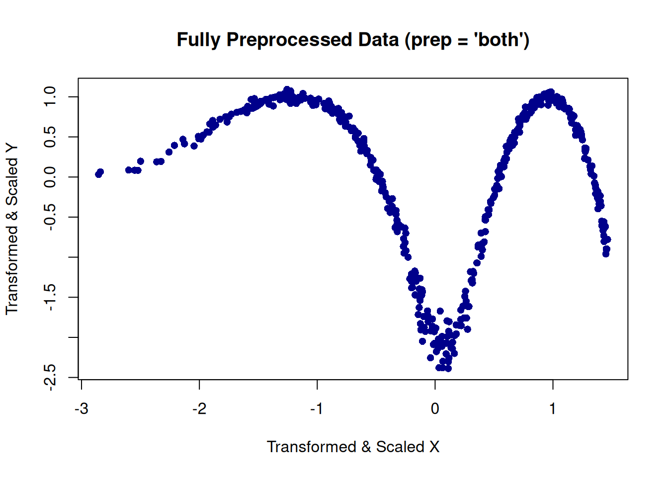
We can quickly inspect the relationship between inputs and targets across preprocessing states:

# Transformed & Scaled State (prep = "both")
plot(
  get_x_all(td, prep = "both"), 
  get_y_all(td, prep = "both"),
  main = "Fully Preprocessed Data (prep = 'both')",
  xlab = "Transformed & Scaled X",
  ylab = "Transformed & Scaled Y",
  col  = "darkblue", 
  pch  = 16
)

Step 2: Building and Compiling the Keras Model

We construct a multi-layer feed-forward neural network using keras_model_sequential(). The network takes 1D scaled inputs, passes them through two hidden dense layers with non-linear activation functions (relu and tanh), and outputs a continuous prediction:

## Construct sequential architecture
model <- keras_model_sequential(input_shape = c(1), input_dtype = "float32") |>
  layer_dense(units = 16, activation = "relu") |>
  layer_dense(units = 16, activation = "tanh") |>
  layer_dense(units = 1)

Downloading uv...Done!

## Compile model with Adam optimizer and Mean Squared Error loss
model |> compile(
  optimizer = optimizer_adam(learning_rate = 0.005),
  loss      = "mse",
  metrics   = c("mae")
)

summary(model)

Model: "sequential"
┏━━━━━━━━━━━━━━━━━━━━━━━━━━━━━━━━━━━┳━━━━━━━━━━━━━━━━━━━━━━━━━━┳━━━━━━━━━━━━━━━┓
┃ Layer (type)                      ┃ Output Shape             ┃       Param # ┃
┡━━━━━━━━━━━━━━━━━━━━━━━━━━━━━━━━━━━╇━━━━━━━━━━━━━━━━━━━━━━━━━━╇━━━━━━━━━━━━━━━┩
│ dense (Dense)                     │ (None, 16)               │            32 │
├───────────────────────────────────┼──────────────────────────┼───────────────┤
│ dense_1 (Dense)                   │ (None, 16)               │           272 │
├───────────────────────────────────┼──────────────────────────┼───────────────┤
│ dense_2 (Dense)                   │ (None, 1)                │            17 │
└───────────────────────────────────┴──────────────────────────┴───────────────┘
 Total params: 321 (1.25 KB)
 Trainable params: 321 (1.25 KB)
 Non-trainable params: 0 (0.00 B)

Step 3: Model Training

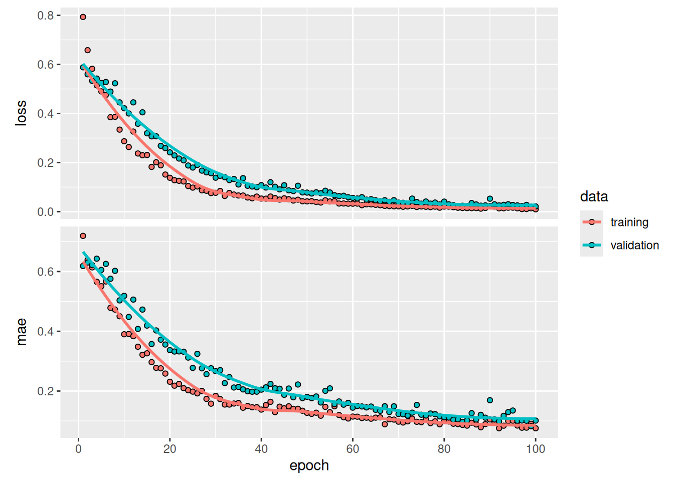
We train the model using get_x_train(td) and get_y_train(td) extracted directly from our td object. Validation splits are specified directly within fit():

history <- model |> fit(
  get_x_train(td), 
  get_y_train(td),
  epochs           = 100,
  batch_size       = 4,
  validation_split = 0.2,
  verbose          = 0
)

plot(history)

Step 4: Model Evaluation on Scaled Space

We can evaluate out-of-sample performance on test data using standard Keras methods or mlfeaturer helpers.

## Keras native evaluation on test set
loss <- evaluate(model, get_x_test(td), get_y_test(td))

13/13 - 0s - 7ms/step - loss: 0.0135 - mae: 0.0898

cat("Test Loss (MSE) =", loss$loss, "\n")

Test Loss (MSE) = 0.01345721

cat("Test MAE        =", loss$mae, "\n")

Test MAE        = 0.08979477

## Using mlfeaturer predict and residual methods
predictions_all  <- predict(td, model, subset = "all")

## not yet implemented for Keras models:
# residuals_all    <- residuals(td, model)

## workaround
residuals_all   <- get_y_all(td, prep = "both") - predictions_all


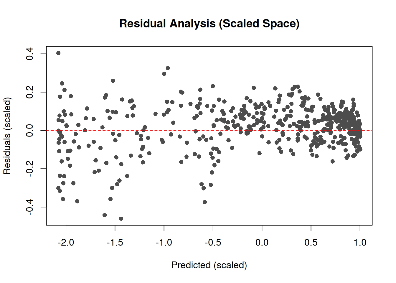
# Scatter plot of predictions vs. residuals on scaled space
plot(
  predictions_all, 
  residuals_all,
  xlab = "Predicted (scaled)",
  ylab = "Residuals (scaled)",
  main = "Residual Analysis (Scaled Space)",
  pch  = 16,
  col  = "gray30"
)
abline(h = 0, col = "red", lty = 2)

Using the qualV package, we can easily compute comprehensive goodness-of-fit metrics across data splits:

## Goodness-of-fit metrics (Jachner et al.)
cat("--- Metrics on Scaled Space ---\n")
cat("Nash-Sutcliffe Efficiency (EF)  =", EF(get_y_all(td), predictions_all), "\n")
cat("R^2 (Train)                     =", rsquared(td, model, subset = "train"), "\n")
cat("R^2 (Test)                      =", rsquared(td, model, subset = "test"), "\n")
cat("R^2 (All)                       =", rsquared(td, model, subset = "all"), "\n")

--- Metrics on Scaled Space ---

Nash-Sutcliffe Efficiency (EF)  = 0.9866436

R^2 (Train)                     = 0.9877619

R^2 (Test)                      = 0.9868988

R^2 (All)                       = 0.9870836

Or a complete set of metrics for the whole data set:

## Goodness-of-fit metrics (Jachner et al.)

# Detailed summary from qualV
compareME(get_y_all(td), predictions_all)

$normalized
                    time    fixed
                    ignore    raw centered scaled ordered
geometry    measure
real        mad            0.1124   0.1045 0.1034  0.1447
            var            0.0133   0.0129 0.0123  0.0105
            sd             0.1155   0.1137 0.1109  0.1023
logarithmic mad               NaN       NA     NA  0.1447
            var               NaN      NaN    NaN  0.0105
            sd                NaN      NaN    NaN  0.1023
geometric   mad               NaN       NA     NA  0.1447
            var               NaN      NaN    NaN  0.0105
            sd                NaN      NaN    NaN  0.1023
ordinal     mad            0.1447   0.1447 0.1447  0.1447
            var            0.0105   0.0105 0.0105  0.0105
            sd             0.1023   0.1023 0.1023  0.1023

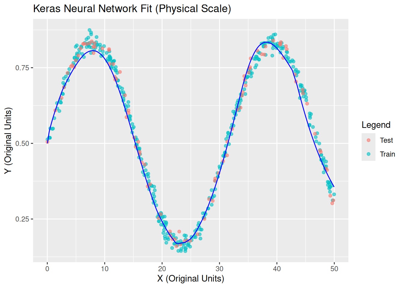
Step 5: Back-Transformation and Evaluation on Physical Scale

A central benefit of mlfeaturer is returning predictions back to original physical units ( $\text{Y}$ ) without writing manual inverse transformations.

We can inspect predictions against raw observations on their original physical scale by setting to_original_scale = TRUE inside predict():

# get predictions for all observed x
y_pred <-
  predict(td, model, to_original_scale = TRUE) |>
  as.data.frame() |>
  rename(y_pred = y)

# plot all original data points and add prediction
get_data(td, prep="none") |>
  mutate(split_label = if_else(split, "Train", "Test")) |>
  as.data.frame() |>
  # add predictions as additional column
  bind_cols(y_pred) |>
  ggplot(aes(x, y)) + 
  geom_point(aes(color = split_label), alpha = 0.6) +
  geom_line(aes(x, y_pred), color = "blue") +
  labs(
    title = "Keras Neural Network Fit (Physical Scale)",
    x     = "X (Original Units)",
    y     = "Y (Original Units)",
    color = "Legend"
  )

Finally, we use ml_evaluate() to calculate overall summary metrics across the pipeline:

ml_evaluate(td, model, to_original_scale = FALSE)

       MSE       RMSE        MAE       BIAS         R2
0.01303548 0.11417303 0.08785710 0.02072296 0.98708364

ml_evaluate(td, model, to_original_scale = TRUE)

         MSE         RMSE          MAE         BIAS           R2
0.0007393892 0.0271917112 0.0221534119 0.0090175801 0.9870649731

Acknowledgments

Many thanks to the R Core Team (R Core Team 2026) for developing and maintaining R. This documentation was written in Quarto (Allaire and Dervieux 2025).

References

Abadi, Martín, Ashish Agarwal, Paul Barham, et al. 2015. TensorFlow: Large-Scale Machine Learning on Heterogeneous Systems. https://www.tensorflow.org/.

Allaire, JJ, and Christophe Dervieux. 2025. Quarto: R Interface to ’Quarto’ Markdown Publishing System. https://doi.org/10.32614/CRAN.package.quarto.

Bradbury, James, Roy Frostig, Peter Hawkins, et al. 2018. JAX: Composable Transformations of Python+NumPy Programs. Released. https://github.com/google/jax.

Kalinowski, Tomasz, JJ Allaire, and François Chollet. 2026. Keras3: R Interface to ’Keras’. https://doi.org/10.32614/CRAN.package.keras3.

Paszke, Adam, Sam Gross, Francisco Massa, et al. 2019. “PyTorch: An Imperative Style, High-Performance Deep Learning Library.” In Advances in Neural Information Processing Systems, edited by H. Wallach, H. Larochelle, A. Beygelzimer, F. d'Alché-Buc, E. Fox, and R. Garnett, vol. 32. Curran Associates, Inc. https://proceedings.neurips.cc/paper_files/paper/2019/file/bdbca288fee7f92f2bfa9f7012727740-Paper.pdf.

R Core Team. 2026. R: A Language and Environment for Statistical Computing. R Foundation for Statistical Computing. https://www.R-project.org/.

03 - Neural Networks with keras