02 - Neural Networks with mlfeaturer and nnet • mlfeaturer

Introduction

In the following, we show how to use mlfeaturer in the context of a simple artificial neural network (ANN) workflow.

The dataset was digitized from figures by Dauta et al. (1990), who analyzed growth rate dependency of four microalgae species on light intensity across different temperatures. We aim to create a regression model to predict specific growth rates ( $\mu$ ) at arbitrary light and temperature values within the measured range.

Note that these data can also be fitted using parametric kinetic models; this alternative approach is covered in a separate tutorial.

Installation

To install the package, first ensure remotes is installed from CRAN, then install mlfeaturer from GitHub:

remotes::install_github("[https://github.com/tpetzoldt/mlfeaturer](https://github.com/tpetzoldt/mlfeaturer)")

Next, load the required packages:

library("mlfeaturer")
library("dplyr")
library("ggplot2")
library("nnet")

Prepare Data

We set up a preprocessed data object dt4 containing the dataset along with its preprocessing specifications.

Before initializing the object with create_preprocessed_data(), we first add dummy variables for the species factor. Because nominal character columns are not directly supported by nnet (Venables and Ripley 2002), we convert species into dummy indicator columns (0 or 1):

# Phytoplankton growth rate dataset
data(dauta4)

spec_dummy <- 
  model.matrix(~ species - 1, dauta4) |>
  as.data.frame()

head(spec_dummy)

  speciesChlorella speciesFragilaria speciesStaurastrum speciesSynechocystis
1                1                 0                  0                    0
2                1                 0                  0                    0
3                1                 0                  0                    0
4                1                 0                  0                    0
5                1                 0                  0                    0
6                1                 0                  0                    0

The original species column and an added row number column (no) are declared as ID columns (id_col). These columns are excluded from modeling inputs and targets but remain accessible for identification and plotting.

Next, we create a random split vector that assigns approximately 60% of observations to the training set and 40% to the test set.

The growthrate column serves as our target ( $y$ ) variable, while all remaining non-ID columns serve as input features ( $X$ ).

For the nnet package (Venables and Ripley 2002), input and output data must be normalized to the $[0, 1]$ interval. Here, we use scale_method = "minmax" with scale_option = "all", deriving min/max bounds from the complete dataset:

dt4 <-
  dauta4 |>
  bind_cols(spec_dummy) |>                     # Add dummy variable columns
  mutate(
    no = 1:n(),
    split = sample(
      c(TRUE, FALSE), 
      n(), 
      prob = c(0.6, 0.4), 
      replace = TRUE
    )
  ) |>
  create_preprocessed_data(
    target_col   = "growthrate",
    id_col       = c("species", "no"),
    split_col    = "split",
    scale_method = "minmax",
    scale_option = "all"                        # Min/max derived from complete dataset
  )

Fit a Neural Network

To fit a neural network with 8 hidden units, we extract the training inputs and target using get_x_train() and get_y_train(). Data are automatically filtered by the split column and scaled according to the minmax method defined in dt4:

net <- nnet(
  get_x_train(dt4), 
  get_y_train(dt4),
  size = 8, 
  maxit = 200, 
  trace = FALSE
)

Evaluate the Network

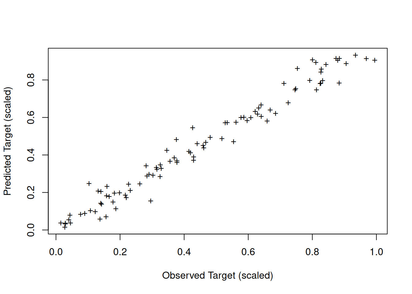
To check whether training converged effectively, we can compare the original scaled targets against scaled model outputs using standard predict() from nnet:

plot(
  get_y_train(dt4), 
  predict(net),
  pch = "+",
  xlab = "Observed Target (scaled)",
  ylab = "Predicted Target (scaled)"
)

The ml_evaluate() helper calculates standard evaluation metrics across the preprocessed data:

ml_evaluate(dt4, net) # Default uses scaled data

        MSE        RMSE         MAE        BIAS          R2
 0.01320042  0.11489309  0.07890552 -0.01673248  0.81053543

We can also calculate performance metrics manually, such as $R^2$ on the training subset:

paste("R^2 (train) =", 1 - var(residuals(net)) / var(get_y_train(dt4)))

[1] "R^2 (train) = 0.969164040334653"

To inspect model performance and detect remaining patterns, we plot residuals across training and test splits:

plot(
  predict(dt4, net), 
  residuals(dt4, net), 
  col = factor(get_data(dt4)[, "split"]),
  xlab = "Predicted (scaled)",
  ylab = "Residuals (scaled)"
)

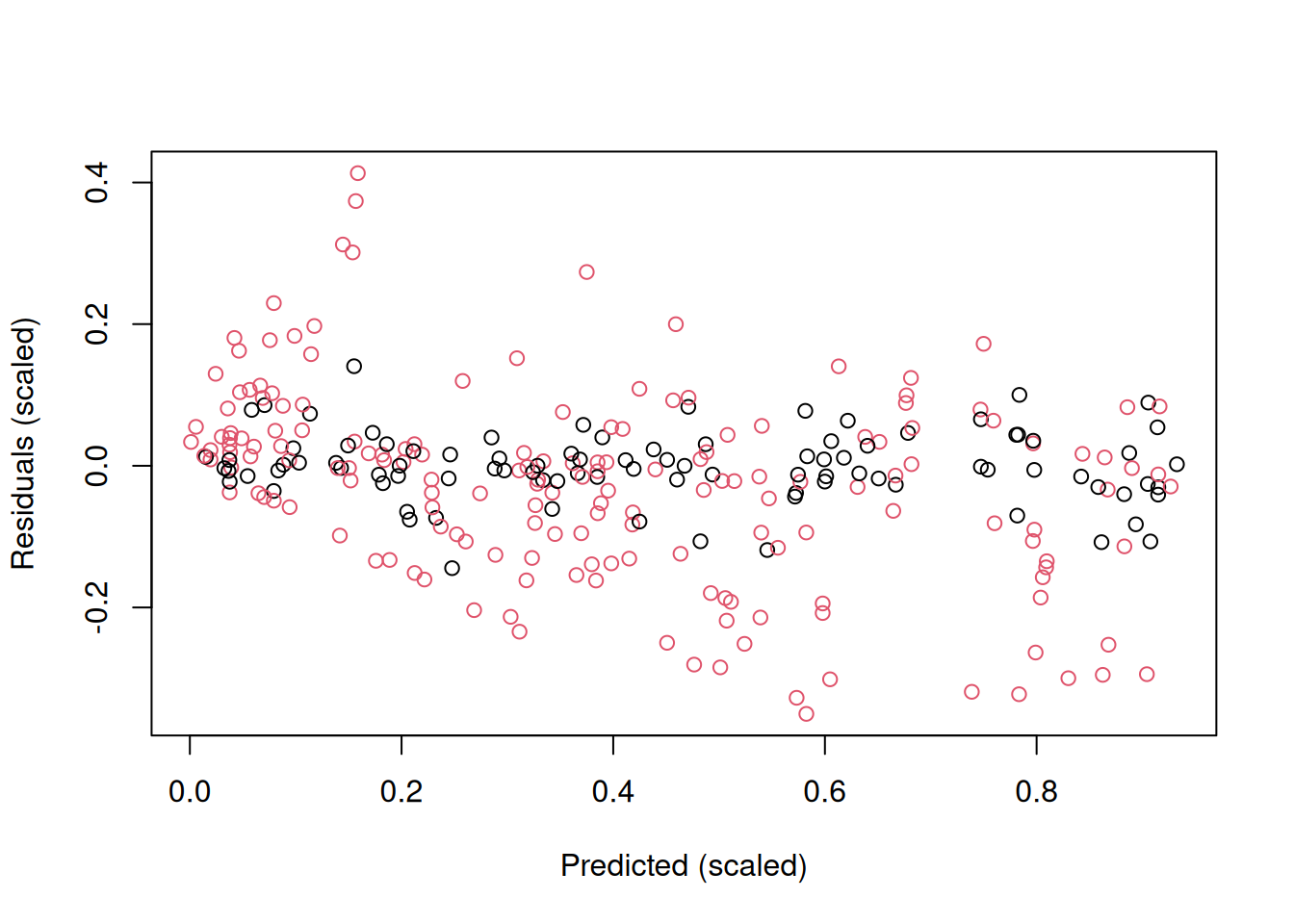
Here, we utilize predict() and residuals() methods provided by mlfeaturer. Unlike standard base methods, these S4 methods take the dt4 container as their first argument to facilitate piping. In the plot above, black points represent the training set and red points represent the test set. Poor out-of-sample performance at higher values often indicates overfitting or sub-optimal random splitting.

Graphical Comparison of Results

First, we evaluate predictions on the scaled/transformed space:

y_pred <-
  predict(dt4, net) |>
  as.data.frame() |>
  rename(growthrate_pred = growthrate)

get_data(dt4) |>
  as.data.frame() |>
  bind_cols(y_pred) |>
  ggplot(aes(light, growthrate)) + 
  geom_point() +
  geom_line(aes(light, growthrate_pred), color = "red") +
  facet_grid(species ~ temperature) +
  labs(title = "Predictions on Scaled Space (prep = 'both')")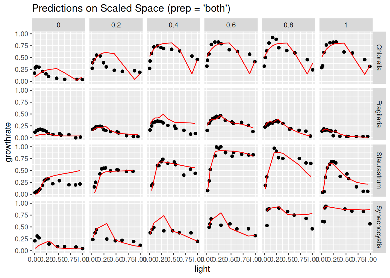

Next, we pass to_original_scale = TRUE to predict() to automatically back-transform predictions to their physical units ( $\text{d}^{-1}$ ), comparing them against raw data extracted via prep = "none":

y_pred_orig_scale <-
  predict(dt4, net, to_original_scale = TRUE) |>
  as.data.frame() |>
  rename(growthrate_pred = growthrate)

get_data(dt4, prep = "none") |>
  as.data.frame() |>
  bind_cols(y_pred_orig_scale) |>
  ggplot(aes(light, growthrate)) + 
  geom_point() +
  geom_line(aes(light, growthrate_pred), color = "red") +
  facet_grid(species ~ temperature) +
  labs(
    title = "Predictions Back-Transformed to Physical Scale (d^-1)",
    x = "Light Intensity",
    y = "Growth Rate (d^-1)"
  )

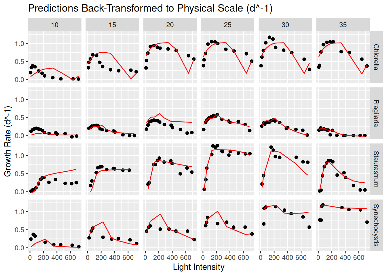
These results serve for demonstration. Out-of-sample accuracy can be significantly improved by increasing optimization epochs, trying multiple random initializations, employing stratified splitting (e.g., across species or temperature strata), or integrating cross-validation.

Acknowledgments

Many thanks to the R Core Team (R Core Team 2026) for developing and maintaining R. This documentation was written in Quarto (Allaire and Dervieux 2025).

References

Allaire, JJ, and Christophe Dervieux. 2025. Quarto: R Interface to ’Quarto’ Markdown Publishing System. https://doi.org/10.32614/CRAN.package.quarto.

Dauta, Alain, Jean Devaux, Françoise Piquemal, and Lhoussaine Boumnich. 1990. “Growth Rate of Four Algae in Relation to Light and Temperature.” Hydrobiologia 207: 221–26. https://doi.org/10.1007/BF00041459.

R Core Team. 2026. R: A Language and Environment for Statistical Computing. R Foundation for Statistical Computing. https://www.R-project.org/.

Venables, W. N., and B. D. Ripley. 2002. Modern Applied Statistics with s. Fourth. Springer. https://www.stats.ox.ac.uk/pub/MASS4/.