01 - Transformation of Features with Package mlfeaturer • mlfeaturer

Introduction

Package mlfeaturer provides lightweight data manipulation support for regression problems with multiple input variables $X$ and a single target variable $y$ . A typical initial task in machine learning is to transform and scale variables, split them into training and test sets, and, after model fitting, compare model outputs against original physical measurements and new evaluation data.

Data preprocessing – such as centering, scaling, and non-linear transformations – is an essential step in building regression models. However, managing scaled and unscaled datasets manually can quickly lead to fragmented code, with multiple copies of data frames (df_scaled, df_train, df_test) and lost transformation parameters.

While comprehensive machine learning frameworks such as recipes (from tidymodels), mlr3, or caret provide robust pipelines for production workflows, they also introduce software overhead, steep learning curves, and deep dependency trees.

mlfeaturer fills the gap between informal scripting and heavy production frameworks. It offers a lightweight, transparent, S4-based system designed specifically for regression workflows.

Core Objectives

mlfeaturer is designed to simplify data handling without interfering with your specific modeling code:

Stateful Feature & Target Preprocessing: Keep track of transformation parameters (e.g., means, standard deviations, custom min/max bounds) directly within dedicated S4 objects.
Seamless Inverse Transformations: Easily back-transform model predictions and target variables to their original physical scales and units for intuitive evaluation, reporting, and plotting.
Train / Test / New Data Consistency: Apply stored transformation parameters deterministically across training splits, test sets, and unscaled new data without data leakage.
Minimal Dependencies: Built with simplicity in mind, ensuring high stability, fast execution, and ease of maintenance.

Target Audience & Use Cases

Teaching & Learning: Serves as a “door-opener” tool for students and researchers learning machine learning fundamentals without the cognitive load of complex pipeline ecosystems.
Domain Science & Applied Research: Intended for environmental scientists, ecologists, and engineers starting with base R models (lm, nls) or classic algorithms (nnet, e1071, randomForest) who need clean target scaling back to physical units.
Lightweight Scripting: Perfect for projects where importing large framework ecosystems is unnecessary or undesirable.

Installation

remotes::install_github("[https://github.com/tpetzoldt/mlfeaturer](https://github.com/tpetzoldt/mlfeaturer)")

Example Workflow: Preprocessing Microalgae Growth Data

To demonstrate how mlfeaturer handles multi-stage preprocessing without creating fragmented data frames, we use the dauta4 dataset included in the package.

The `dauta4` Dataset

The dauta4 dataset originates from laboratory experiments conducted by Dauta et al. (1990) investigating the combined effects of light intensity and temperature on the specific growth rates of various freshwater microalgae species.

The dataset contains four key variables: - species: Microalgae species identifier. - light: Irradiance levels (e.g., $\mu\text{mol m}^{-2}\text{s}^{-1}$ ). - temperature: Water temperature (°C). - growthrate: Specific growth rate ( $\text{d}^{-1}$ ), serving as our target variable ( $y$ ).

Step 1: Scaling and Transformation Pipeline

In regression modeling—especially with non-linear methods like artificial neural networks or support vector machines—inputs ( $X$ ) and targets ( $y$ ) often require scaling (e.g., min-max normalization to $[0, 1]$ ) as well as domain-specific non-linear transformations (e.g., log-transforms for kinetics or square-root/square transforms for variance stabilization).

With mlfeaturer, all transformations and scaling parameters are declared in a single, stateful container (dt4 in the dauta4 example) via create_preprocessed_data():

library("mlfeaturer")
library("dplyr")
library("ggplot2")

data(dauta4)

## Scaling and transformation pipeline ========================================
dt4 <-
  dauta4 |>
  mutate(species = as.numeric(species)) |>
  create_preprocessed_data(
    target_col   = "growthrate",
    scale_method = "minmax",
    scale_option = "all",
    fun_transform = list(
      light       = \(x) 0.1 * x,
      temperature = \(x) log(x),
      growthrate  = \(x) x^2
    )
  )

Notice how fun_transform accepts a list of transformation functions using R’s anonymous function syntax (\(x)).

Step 2: Extracting Preprocessing States

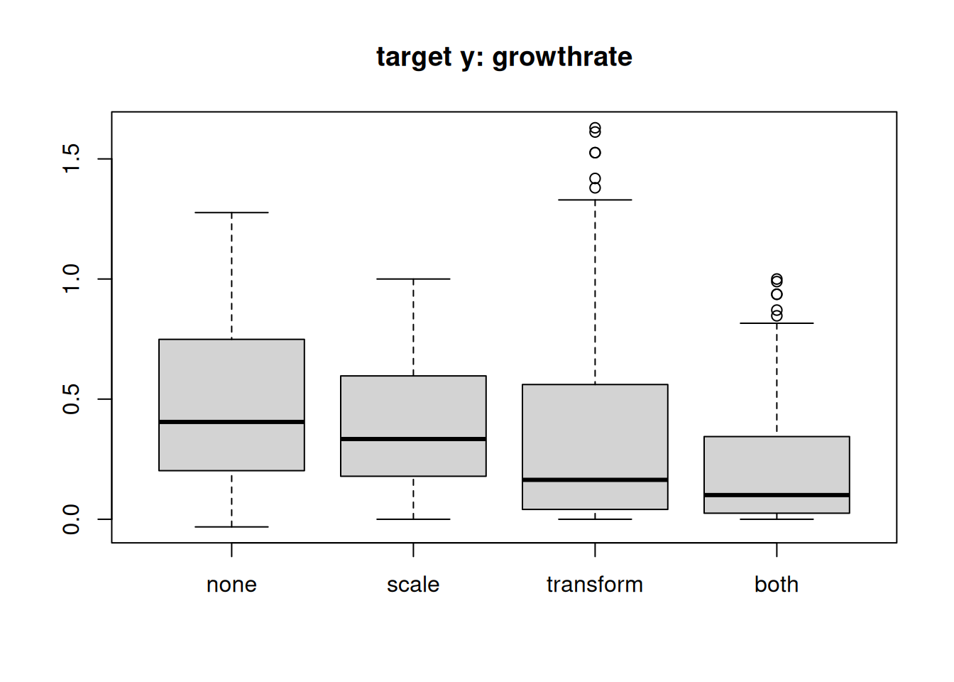
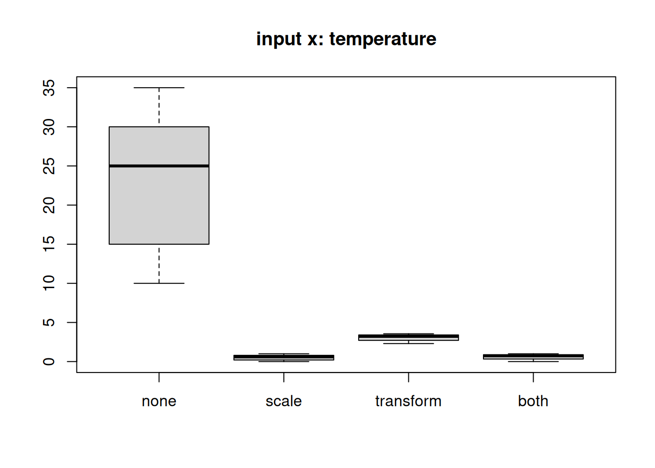
A core advantage of mlfeaturer is that the original data, scaled data, transformed data, and fully preprocessed data (both) all remain accessible from the single dt4 object using extractor functions like get_y_all(), get_x_all(), and get_data().

The prep argument accepts four states: 1. "none": Original raw data. 2. "scale": Data with scaling applied. 3. "transform": Data with non-linear function transformations applied. 4. "both": Data with both transformations and scaling applied.

We can inspect how the distributions change across these stages using standard boxplots:

# Target variable (y) comparison
boxplot(
  tibble(
    none      = get_y_all(dt4, prep = "none"),
    scale     = get_y_all(dt4, prep = "scale"),
    transform = get_y_all(dt4, prep = "transform"),
    both      = get_y_all(dt4, prep = "both")
  ),
  main = "target y: growthrate"
)

Boxplots comparing target growthrate and input temperature across preprocessing states

# Input variable (x) comparison: temperature
boxplot(
  tibble(
    none      = get_x_all(dt4, prep = "none")[, "temperature"],
    scale     = get_x_all(dt4, prep = "scale")[, "temperature"],
    transform = get_x_all(dt4, prep = "transform")[, "temperature"],
    both      = get_x_all(dt4, prep = "both")[, "temperature"]
  ),
  main = "input x: temperature"
)

Step 3: Visualizing Relationships Across Preprocessing States

By passing prep directly into get_data(), we can generate ggplot2 visualizations for each stage of the dataset without cluttering the workspace with temporary data frames:

# 1. Original raw data
get_data(dt4, prep = "none") |>
  ggplot(aes(light, growthrate)) + 
  geom_point() + 
  facet_grid(species ~ temperature) +
  labs(title = "Raw Data (prep = 'none')")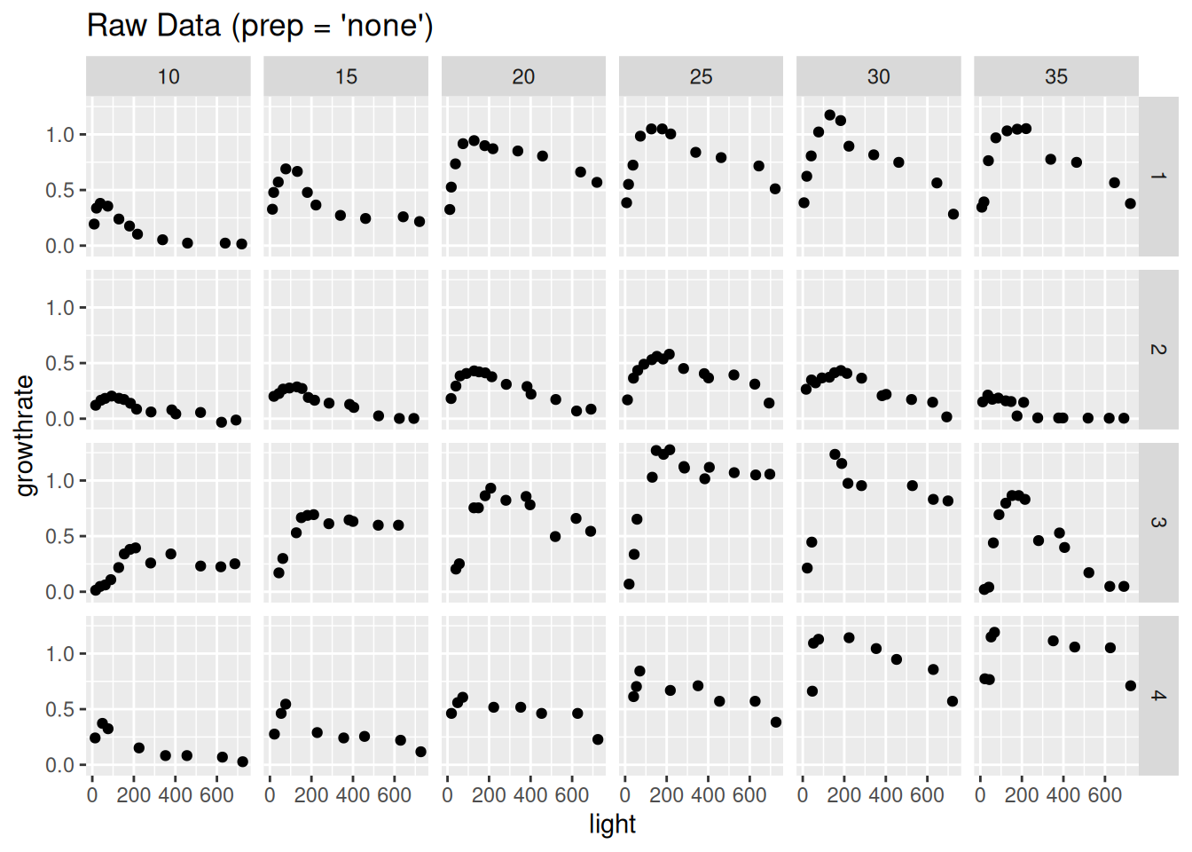

# 2. Scaled data
get_data(dt4, prep = "scale") |>
  ggplot(aes(light, growthrate)) + 
  geom_point() + 
  facet_grid(species ~ temperature) +
  labs(title = "Scaled Data (prep = 'scale')")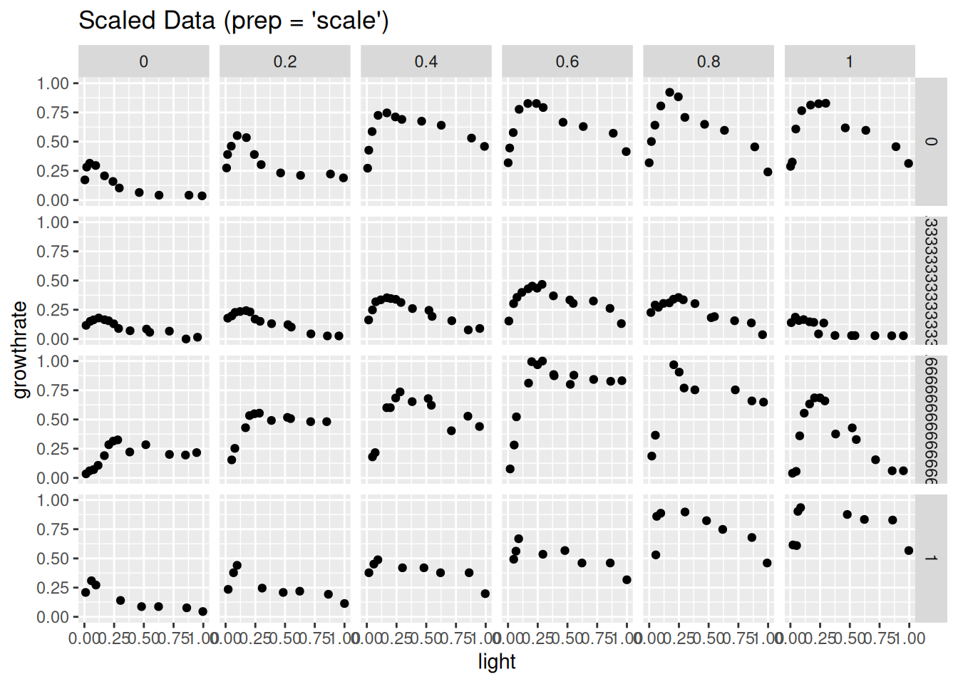

# 3. Transformed data
get_data(dt4, prep = "transform") |>
  ggplot(aes(light, growthrate)) + 
  geom_point() + 
  facet_grid(species ~ temperature) +
  labs(title = "Transformed Data (prep = 'transform')")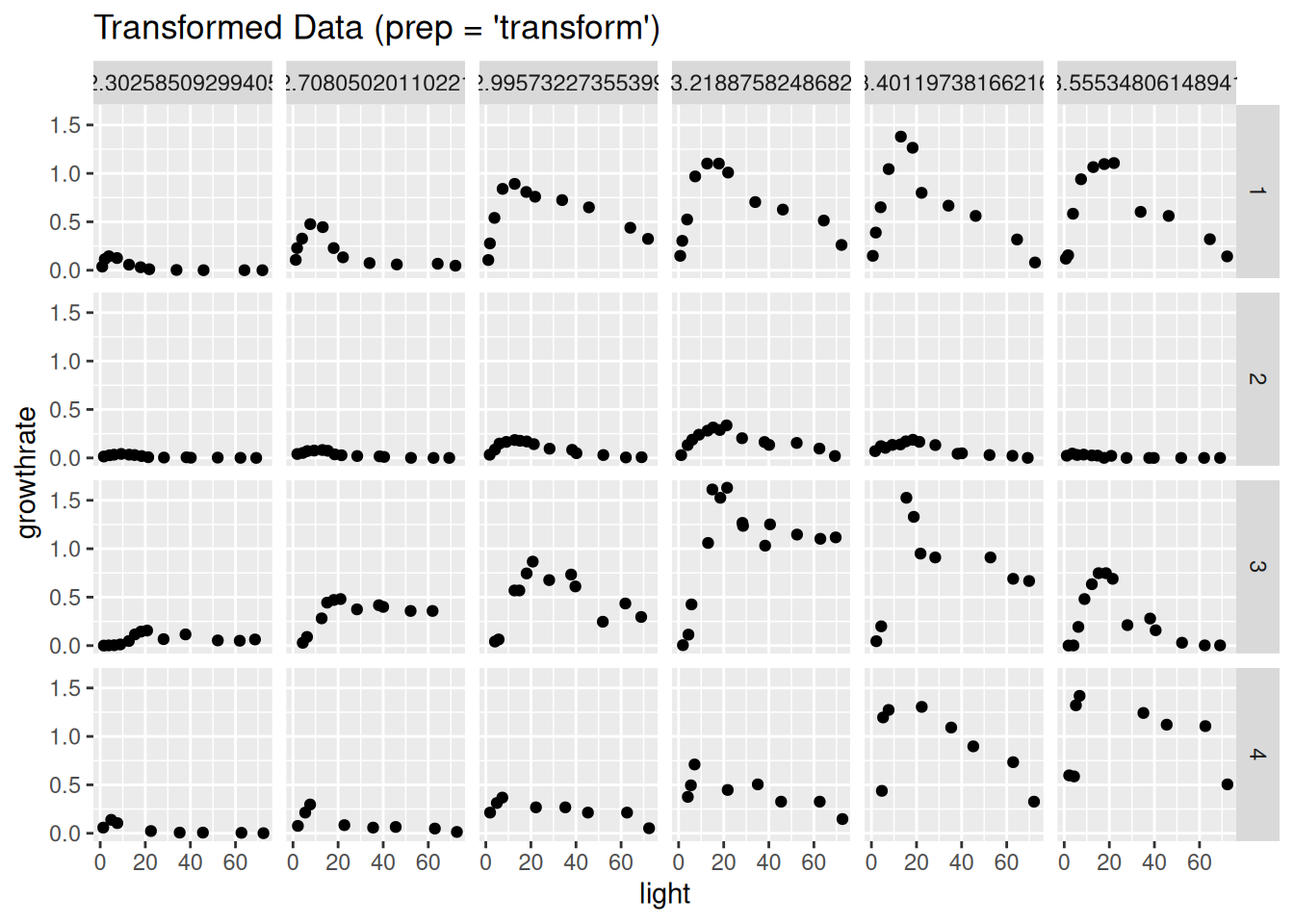

# 4. Fully preprocessed data (both transform & scale)
get_data(dt4, prep = "both") |>
  ggplot(aes(light, growthrate)) + 
  geom_point() + 
  facet_grid(species ~ temperature) +
  labs(title = "Fully Preprocessed Data (prep = 'both')")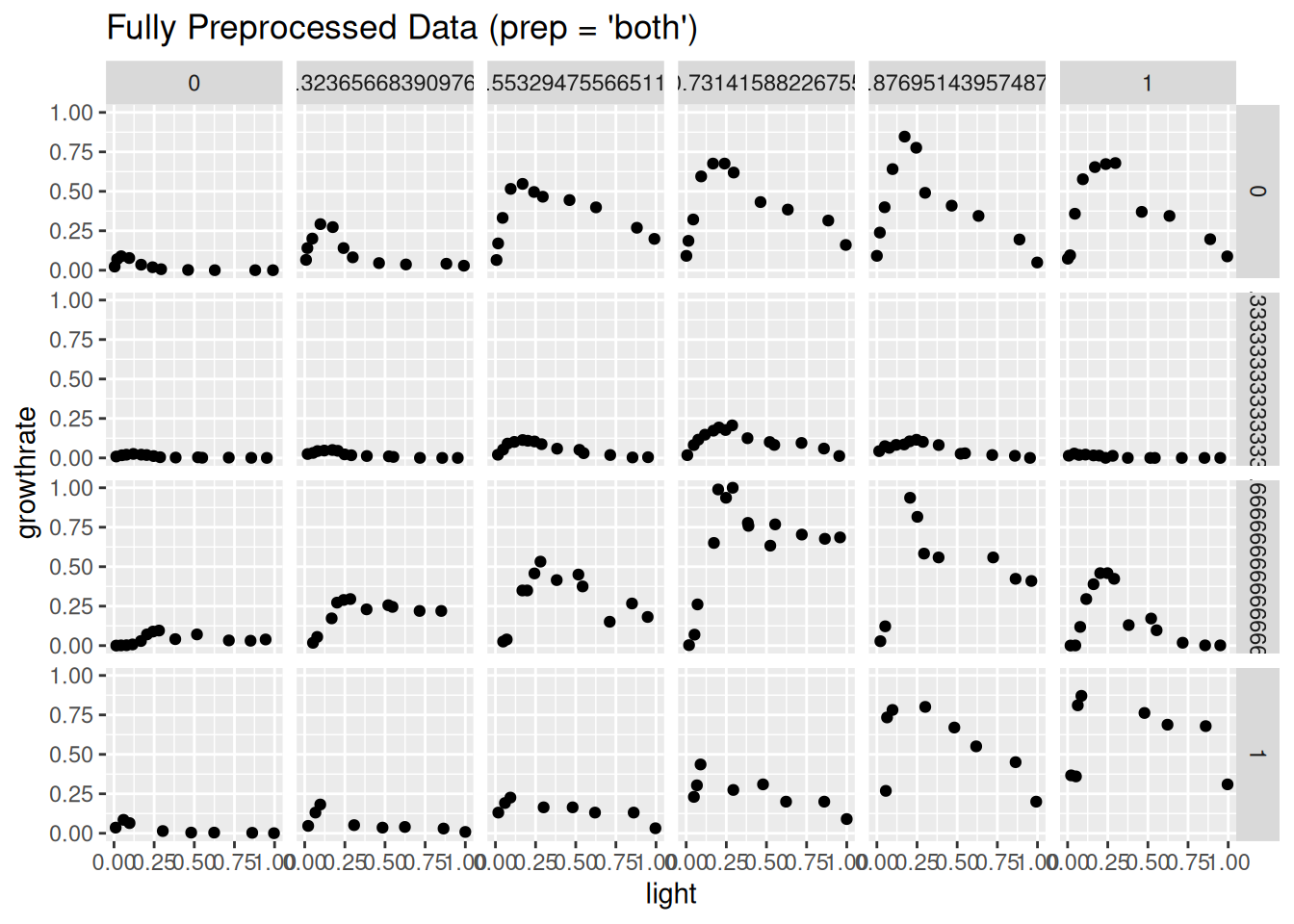

Step 4: Model Fitting and Prediction Back-Transformation

Once features and target variables are preprocessed, model fitting proceeds directly using the preprocessed matrices or data frames.

For instance, we can fit a simple neural network using nnet::nnet (Venables and Ripley 2002) on the fully transformed and scaled data (prep = "both"):

library("nnet")

# Fit neural network on fully preprocessed inputs and target
x_train <- get_x_all(dt4, prep = "both")
y_train <- get_y_all(dt4, prep = "both")

fit <- nnet(x_train, y_train, size = 5, linout = TRUE, trace = FALSE)

# Predict on the fully preprocessed scale (prep = "both")
y_pred_scaled <- predict(fit, x_train)

# Back-transform predictions to the original physical scale (growthrate in d^-1)
y_pred_orig <- inv_transform_data(dt4, y_pred_scaled)

Step 5: Evaluating Model Predictions on Physical Scale

Because inv_transform_data() returns a feature_data object, we can extract the back-transformed predictions on the original physical scale using get_y_all(y_pred_orig, prep = "none").

First, let’s examine the actual versus predicted values on a simple scatter plot:

# Compare actual vs predicted on original physical scale (d^-1)
df_eval <- tibble(
  actual    = get_y_all(dt4, prep = "none"),
  predicted = get_y_all(y_pred_orig, prep = "none")
)

df_eval |>
  ggplot(aes(x = actual, y = predicted)) +
  geom_point(alpha = 0.7) +
  geom_abline(intercept = 0, slope = 1, linetype = "dashed", color = "red") +
  labs(
    title = "Neural Network Predictions vs. Observed Growth Rate",
    x     = "Observed Growth Rate (d^-1)",
    y     = "Predicted Growth Rate (d^-1)"
  ) +
  theme_bw()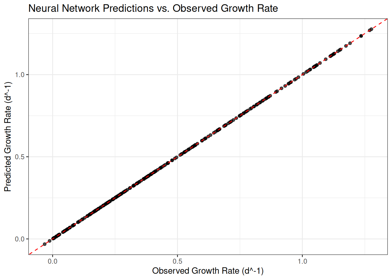

While the scatter plot shows strong overall agreement, visualizing the response curves across experimental conditions (light and temperature per species) reveals how well the model captures the underlying biological kinetics:

# Combine original unscaled data with back-transformed predictions
df_curves <- get_data(dt4, prep = "none") |>
  as.data.frame() |>
  bind_cols(growthrate_pred = get_y_all(y_pred_orig, prep = "none"))

df_curves |>
  ggplot(aes(x = light, y = growthrate)) +
  geom_point(aes(color = "Observed"), alpha = 0.8) +
  geom_line(aes(y = growthrate_pred, color = "Predicted"), linewidth = 0.8) +
  facet_grid(species ~ temperature, labeller = label_both) +
  scale_color_manual(values = c("Observed" = "black", "Predicted" = "red")) +
  labs(
    title = "Observed Growth Rates vs. Neural Network Response Curves",
    x     = "Light Intensity",
    y     = "Growth Rate (d^-1)",
    color = "Legend"
  ) +
  theme_bw() +
  theme(legend.position = "top")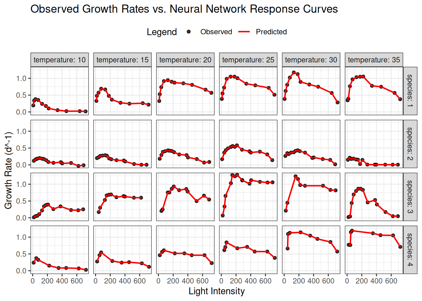

The near-perfect match between predictions and observations is a classic hallmark of neural networks: when trained on the full dataset without regularization or early stopping, functions like nnet::nnet can easily overfit and near-perfectly memorize the training points, resulting in a suspiciously tight actual-vs-predicted plot.

How to properly prevent overfitting using train/test splitting and validation workflows with mlfeaturer is explained in the next vignette, “02 - Neural Networks with mlfeaturer and nnet” (02-ann-simple.qmd).

Summary & Next Steps

mlfeaturer eliminates the need to manage scattered copies of data frames during regression analysis. By encapsulating scaling parameters and non-linear transformation functions inside a single S4 object, it allows straightforward transitions between normalized feature spaces during training and physical scales during evaluation.

For advanced examples—including train/test splitting routines and cross-validation workflows—refer to the additional vignettes and scripts in the inst/doc/examples directory of the package repository.

Acknowledgments

Many thanks to the R Core Team (R Core Team 2026) for developing and maintaining R. This documentation was written in Quarto (Allaire and Dervieux 2025).

References

Allaire, JJ, and Christophe Dervieux. 2025. Quarto: R Interface to ’Quarto’ Markdown Publishing System. https://doi.org/10.32614/CRAN.package.quarto.

Dauta, Alain, Jean Devaux, Françoise Piquemal, and Lhoussaine Boumnich. 1990. “Growth Rate of Four Algae in Relation to Light and Temperature.” Hydrobiologia 207: 221–26. https://doi.org/10.1007/BF00041459.

R Core Team. 2026. R: A Language and Environment for Statistical Computing. R Foundation for Statistical Computing. https://www.R-project.org/.

Venables, W. N., and B. D. Ripley. 2002. Modern Applied Statistics with s. Fourth. Springer. https://www.stats.ox.ac.uk/pub/MASS4/.

01 - Transformation of Features with Package mlfeaturer