x1-R Basics

Applied Statistics – A Practical Course

Thomas Petzoldt

2024-08-23

Prerequisites

1. Install R 4.x from the CRAN server: e.g. https://cloud.r-project.org/
2. Install a recent version of RStudio: https://posit.co/download/rstudio-desktop/

• R and RStudio are available for Linux, Windows and MacOS
• Install R first and RStudio second

Outline

1. Expressions and assignments
2. Elements of the R language
3. Data objects: vectors, matrices, algebra
4. Data import
5. Lists
6. Loops and conditional execution
7. Further reading

R is more convenient with RStudio

R and RStudio

Engine and Control

• R The main engine for computations and graphics.
• Rstudio the IDE (integrated development environment) that embeds and controls R and provides additional facilities.
• R can also be used without RStudio.

Citation

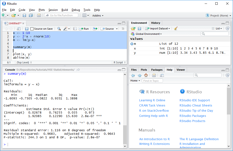
Cite R and optionally RStudio.

R Core Team (2022). R: A language and environment for statistical computing. R Foundation for Statistical Computing, Vienna, Austria. https://www.R-project.org/

RStudio Team (2022). RStudio: Integrated Development Environment for R. RStudio, PBC, Boston, MA URL http://www.rstudio.com/

Elements of the R language

Expressions and Assignments

Expression

1 - pi + exp(1.7)

[1] 3.332355

• result is printed to the screen
• the [1] indicates that the value shown at the beginning of the line is the first (and here the only) element

Assignment

a <- 1 - pi + exp(1.7)

• The expression on the left hand side is assigned to the variable on the right.
• The arrow is spelled as “a gets …”
• To avoid confusion: use <- for assignment and let = for parameter matching

Constants, variables and assignments

Assignment of constants and variables to a variable

x <- 1.3      # numeric constant
y <- "hello"  # character constant
a <- x        # a and x both variables

Assignment in opposite direction (rarely used)

x -> b

Multiple assignment

x <- a <- b

Do not use the following constructs

# Equal sign has two meanings: parameter matching and assignment
# - Don't use it for assignment!
x = a

# Super assignment, useful for programmers in special cases
x <<- 2 

Objects, constants, variables

• Everything stored in R’s memory is an object:
  • can be simple or complex
  • can be constants or variables
  • constants: 1, 123, 5.6, 5e7, “hello”
  • variables: can change their value, are referenced by variable names

x <- 2.0 # x is a variable, 2.0 is a constant

A syntactically valid variable name consists of:

• letters, numbers, underline (_), dot (.)
• starts with a letter or the dot
• if starting with the dot, not followed by a number

Special characters, except _ and . (underscore and dot) are not allowed.

International characters (e.g German umlauts ä, ö, ü, …) are possible, but not recommended.

Allowed and disallowed identifiers

correct:

• x, y, X, x1, i, j, k
• value, test, myVariableName, do_something
• `.hidden, .x1``

forbidden:

• 1x, .1x (starts with a number)
• !, @, \$, #, space, comma, semicolon and other special characters

reserved words cannot be used as variable names:

• if, else, repeat, while, function, for, in, next, break
• TRUE, FALSE, NULL, Inf, NaN, NA, NA_integer_, NA_real_, NA_complex_, NA_character\_
• ..., ..1, ..2

Note: R is case sensitive, x and X, value and Value are different.

Operators

operator	symbol
Addition	+
Subtraction	-
Negation	-
Multiplication	*
Division	/
Modulo	%%
Integer Divison	%/%
Power	^
Matrix product	%*%
Outer product	%o%

operator	symbol
Negation	!
And	&
Or	|
Equal	==
Unequal	!=
Less than	<
Greater than	>
Less or equal	<=
Greater or equal	>=
Assignment	<-
Element of a list	$
Pipeline	|>

… and more

Functions

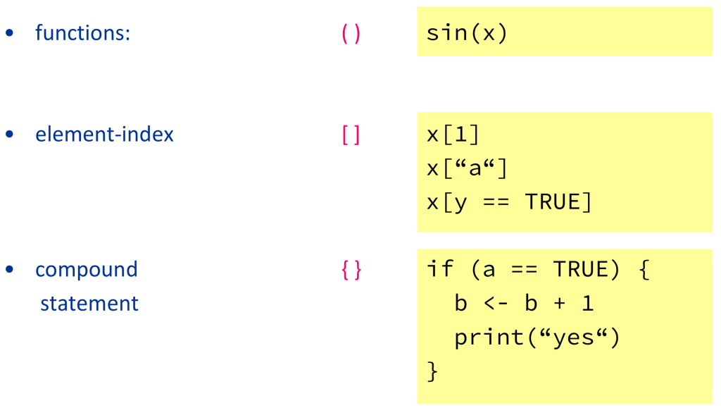
Pre-defined functions:

• with return value: sin(x), log(x)
• with side effect: plot(x), print(x)
• with both return value and side efect: hist(x)

Arguments: mandatory or optional, un-named or named

• plot(1:4, c(3, 4, 3, 6), type = "l", col = "red")
• if named arguments are used (with the “=” sign), argument order does not matter

User-defined functions:

• can be used to extend R
• will be discussed later

\(\rightarrow\) Functions have always a name followed by arguments in round parentheses.

Parentheses

Data objects

• different classes: vector, matrix, list, data.frame, …
• content: numbers, text, maps, sound, images, videos.

We start with vectors, matrices and arrays, and data frames.

Vectors, matrices and arrays

• vectors = 1D, matrices = 2D and arrays = n-dimensional

• data are arranged into rows, columns, layers, …

• data filled in column-wise, can be changed

• create vector

x <- 1:20
x

 [1]  1  2  3  4  5  6  7  8  9 10 11 12 13 14 15 16 17 18 19 20

• convert it to matrix

y <- matrix(x, nrow = 5, ncol = 4)
y

     [,1] [,2] [,3] [,4]
[1,]    1    6   11   16
[2,]    2    7   12   17
[3,]    3    8   13   18
[4,]    4    9   14   19
[5,]    5   10   15   20

• back-convert (flatten) to vector

as.vector(y) # flattens the matrix to a vector

 [1]  1  2  3  4  5  6  7  8  9 10 11 12 13 14 15 16 17 18 19 20

Vectors, matrices and arrays II

• recycling rule if the number of elements is too small

x <- matrix(0, nrow=5, ncol=4)
x

     [,1] [,2] [,3] [,4]
[1,]    0    0    0    0
[2,]    0    0    0    0
[3,]    0    0    0    0
[4,]    0    0    0    0
[5,]    0    0    0    0

x <- matrix(1:4, nrow=5, ncol=4)
x

     [,1] [,2] [,3] [,4]
[1,]    1    2    3    4
[2,]    2    3    4    1
[3,]    3    4    1    2
[4,]    4    1    2    3
[5,]    1    2    3    4

Transpose rows and columns

• row-wise creation of a matrix

x <- matrix(1:20, nrow = 5, ncol = 4, byrow = TRUE)
x

     [,1] [,2] [,3] [,4]
[1,]    1    2    3    4
[2,]    5    6    7    8
[3,]    9   10   11   12
[4,]   13   14   15   16
[5,]   17   18   19   20

• transpose of a matrix

x <- t(x)
x

     [,1] [,2] [,3] [,4] [,5]
[1,]    1    5    9   13   17
[2,]    2    6   10   14   18
[3,]    3    7   11   15   19
[4,]    4    8   12   16   20

Access array elements

• a three dimensional array
• row, column, layer/page
• sub-matrices (slices)

x <- array(1:24, dim=c(3, 4, 2))
x

, , 1

     [,1] [,2] [,3] [,4]
[1,]    1    4    7   10
[2,]    2    5    8   11
[3,]    3    6    9   12

, , 2

     [,1] [,2] [,3] [,4]
[1,]   13   16   19   22
[2,]   14   17   20   23
[3,]   15   18   21   24

• elements of a matrix or array

x[1, 3, 1] # single element

[1] 7

x[ , 3, 1] # 3rd column of 1st layer

[1] 7 8 9

x[ ,  , 2] # second layer

     [,1] [,2] [,3] [,4]
[1,]   13   16   19   22
[2,]   14   17   20   23
[3,]   15   18   21   24

x[1,  ,  ] # another slice

     [,1] [,2]
[1,]    1   13
[2,]    4   16
[3,]    7   19
[4,]   10   22

Reordering and indirect indexing

Original matrix

(x <- matrix(1:20, nrow = 4))

     [,1] [,2] [,3] [,4] [,5]
[1,]    1    5    9   13   17
[2,]    2    6   10   14   18
[3,]    3    7   11   15   19
[4,]    4    8   12   16   20

Inverted row order

x[4:1, ]

     [,1] [,2] [,3] [,4] [,5]
[1,]    4    8   12   16   20
[2,]    3    7   11   15   19
[3,]    2    6   10   14   18
[4,]    1    5    9   13   17

Indirect index

x[c(1, 2, 1, 2), c(1, 3, 2, 5, 4)]

     [,1] [,2] [,3] [,4] [,5]
[1,]    1    9    5   17   13
[2,]    2   10    6   18   14
[3,]    1    9    5   17   13
[4,]    2   10    6   18   14

Logical selection

x[c(FALSE, TRUE, FALSE, TRUE), ]

     [,1] [,2] [,3] [,4] [,5]
[1,]    2    6   10   14   18
[2,]    4    8   12   16   20

Surprise?

x[c(0, 1, 0, 1), ]

     [,1] [,2] [,3] [,4] [,5]
[1,]    1    5    9   13   17
[2,]    1    5    9   13   17

Matrix algebra

Matrix

(x <- matrix(1:4,   nrow = 2))

     [,1] [,2]
[1,]    1    3
[2,]    2    4

Diagonal matrix

(y <- diag(2))

     [,1] [,2]
[1,]    1    0
[2,]    0    1

Element wise addition and multiplication

x * (y + 1)

     [,1] [,2]
[1,]    2    3
[2,]    2    8

Outer product (and sum)

1:4 %o% 1:4

     [,1] [,2] [,3] [,4]
[1,]    1    2    3    4
[2,]    2    4    6    8
[3,]    3    6    9   12
[4,]    4    8   12   16

outer(1:4, 1:4, FUN = "+")

     [,1] [,2] [,3] [,4]
[1,]    2    3    4    5
[2,]    3    4    5    6
[3,]    4    5    6    7
[4,]    5    6    7    8

Matrix multiplication

x %*% y

     [,1] [,2]
[1,]    1    3
[2,]    2    4

Matrix multiplication explained

Two matrices: A and B

A <- matrix(c(1, 2, 3,
              5, 4, 2), 
            nrow = 2, byrow = TRUE)

B <- matrix(c(1, 2, 3, 4,
              6, 8, 4, 2,
              3, 1, 3, 2), 
            nrow = 3, byrow = TRUE)

Multiplication: \(A \cdot B\)

A %*% B

     [,1] [,2] [,3] [,4]
[1,]   22   21   20   14
[2,]   35   44   37   32

Transpose and inverse

Matrix

X <- matrix(c(1, 2, 3, 
              4, 3, 2, 
              5, 4, 6),
            nrow = 3)
X

     [,1] [,2] [,3]
[1,]    1    4    5
[2,]    2    3    4
[3,]    3    2    6

Transpose

t(X)

     [,1] [,2] [,3]
[1,]    1    2    3
[2,]    4    3    2
[3,]    5    4    6

Inverse (\(X^{-1}\))

solve(X)

        [,1]    [,2]    [,3]
[1,] -0.6667  0.9333 -0.0667
[2,]  0.0000  0.6000 -0.4000
[3,]  0.3333 -0.6667  0.3333

Multiplication of a matrix with its inverse

\[X \cdot X^{-1} = I\]

X %*% solve(X)

     [,1] [,2] [,3]
[1,]    1    0    0
[2,]    0    1    0
[3,]    0    0    1

\(I\): identity matrix

Linear system of equations

\[\begin{align} 3x && + && 2y && - && z && = && 1 \\ 2x && - && 2y && + && 4z && = && -2 \\ -x && + && 1/2y && - && z && = && 0 \end{align}\]

A <- matrix(c(3,  2,   -1,
             2,  -2,    4,
            -1,   0.5, -1), nrow=3, byrow=TRUE)
b <- c(1, -2, 0)

\[\begin{align} Ax &= b\\ x &= A^{-1}b \end{align}\]

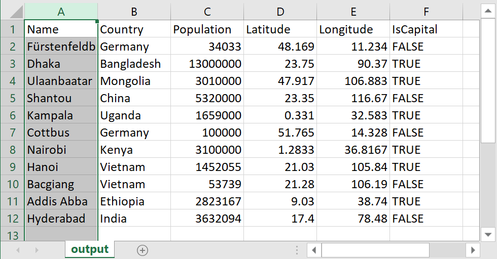
solve(A) %*% b

     [,1]
[1,]    1
[2,]   -2
[3,]   -2

Data frames and data import

Data frames

• represent tabular data
• similar to matrices, but different types of data in columns possible
• typically imported from a file with read.table or read.csv

cities <- read.csv("cities.csv")
cities

               Name    Country Population Latitude Longitude IsCapital
1  Fürstenfeldbruck    Germany      34033  48.1690   11.2340     FALSE
2             Dhaka Bangladesh   13000000  23.7500   90.3700      TRUE
3       Ulaanbaatar   Mongolia    3010000  47.9170  106.8830      TRUE
4           Shantou      China    5320000  23.3500  116.6700     FALSE
5           Kampala     Uganda    1659000   0.3310   32.5830      TRUE
6           Cottbus    Germany     100000  51.7650   14.3280     FALSE
7           Nairobi      Kenya    3100000   1.2833   36.8167      TRUE
8             Hanoi    Vietnam    1452055  21.0300  105.8400      TRUE
9          Bacgiang    Vietnam      53739  21.2800  106.1900     FALSE
10       Addis Abba   Ethiopia    2823167   9.0300   38.7400      TRUE
11        Hyderabad      India    3632094  17.4000   78.4800     FALSE

\(\rightarrow\) download data set

What is a CSV file?

• comma separated values.
• first line contains column names
• decimal is dec=".", column separator is sep=","

Example CSV file (Data from Wikipedia, 2023)

Name,Country,Population,Latitude,Longitude
Dhaka,Bangladesh,10278882,23.75,90.37
Ulaanbaatar,Mongolia,1672627,47.917,106.883
Shantou,China,5502031,23.35,116.67
Kampala,Uganda,1680600,0.331,32.583
Berlin,Germany,3850809,52.52,13.405
Nairobi,Kenya,4672000,1.2833,36.8167
Hanoi,Vietnam,8435700,21.03,105.84
Addis Abba,Ethiopia,3945000,9.03,38.74
Hyderabad,India,9482000,17.4,78.48

Hints

• some countries use dec = "," and sep = ";"
• Excel may export mixed style with dec = "." and sep = ";"
• comments above the header line can be skipped

Different read-Funktions

• R contains several read-functions for different file types.
• Some are more flexible, some more automatic, some faster, some more robust …

To avoid confusion, we use only the following:

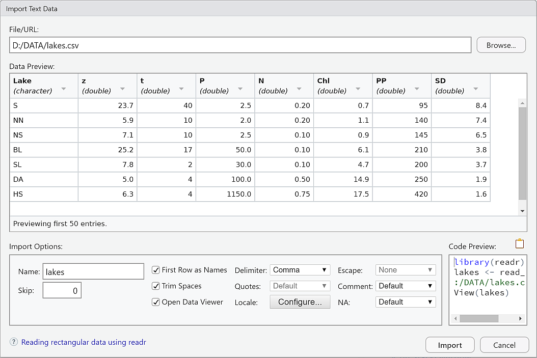
Base R

• read.table(): this is the most flexible standard function, see help file for details
• read.csv(): default options for standard csv files (with dec="." and sep=,)

Tidyverse readr-package

• read_delim(): similar to read.table() but more modern, automatic and faster
• read_csv(): similar to read.csv() with more automatism, e.g. date detection

The most versatile: read.table()

read.table(file, header = FALSE, sep = "", quote = "\"'",
           dec = ".", numerals = c("allow.loss", "warn.loss", "no.loss"),
           row.names, col.names, as.is = !stringsAsFactors, tryLogical = TRUE,
           na.strings = "NA", colClasses = NA, nrows = -1,
           skip = 0, check.names = TRUE, fill = !blank.lines.skip,
           strip.white = FALSE, blank.lines.skip = TRUE,
           comment.char = "#",
           allowEscapes = FALSE, flush = FALSE,
           stringsAsFactors = FALSE,
           fileEncoding = "", encoding = "unknown", text, skipNul = FALSE)

Examples

read.table("cities.csv", sep = ",",  dec = ".")  # same as read.csv
read.table("cities.txt", sep = "\t", dec = ".")  # tab delimited
read.table("cities.csv", sep = ";",  dec = ",")  # German csv

read.table("cities.csv", sep = ",", dec = ".", skip = 5) # skip first 5 lines

Recommendation

Most of our course examples are plain CSV files, so we can use read.csv() or read_csv().

library("readr")
cities <- read_csv("cities.csv")
cities

# A tibble: 11 × 6
   Name             Country    Population Latitude Longitude IsCapital
   <chr>            <chr>           <dbl>    <dbl>     <dbl> <lgl>    
 1 Fürstenfeldbruck Germany         34033   48.2        11.2 FALSE    
 2 Dhaka            Bangladesh   13000000   23.8        90.4 TRUE     
 3 Ulaanbaatar      Mongolia      3010000   47.9       107.  TRUE     
 4 Shantou          China         5320000   23.4       117.  FALSE    
 5 Kampala          Uganda        1659000    0.331      32.6 TRUE     
 6 Cottbus          Germany        100000   51.8        14.3 FALSE    
 7 Nairobi          Kenya         3100000    1.28       36.8 TRUE     
 8 Hanoi            Vietnam       1452055   21.0       106.  TRUE     
 9 Bacgiang         Vietnam         53739   21.3       106.  FALSE    
10 Addis Abba       Ethiopia      2823167    9.03       38.7 TRUE     
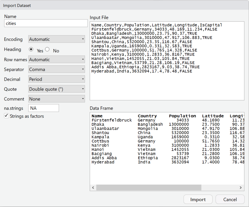
11 Hyderabad        India         3632094   17.4        78.5 FALSE    

Data import assistant of RStudio

File –> Import Dataset

Several options are available:

• “From text (base)” uses the classical R functions
• “From text (readr)” is more modern and uses an add-on package
• “From Excel” can read Excel files if (and only if) they have a clear tabular structure

From text (base)

From text (readr)

Save data to Excel-compatible format

English number format (“.” as decimal):

write.table(cities, "output.csv", row.names = FALSE, sep=",")

German number format (“,” as decimal):

write.table(cities, "output.csv", row.names = FALSE, sep=";", dec=",")

## Creation of data frames

• typical: read data from external file, e.g. csv-files.
• small data frames can be created inline in a script

Inline creation of a data frame

clem <- data.frame(
  brand = c("EP", "EB", "EB", "EB", "EB", "EB", "EB", "EB", "EB", "EB", "EB", 
            "EB", "EB", "EB", "EP", "EP", "EP", "EP", "EP", "EP", "EP", "EB", "EP"),
  weight = c(88, 96, 100, 96, 90, 100, 92, 92, 102, 99, 86, 89, 99, 89, 75, 80, 
             81, 96, 82, 98, 80, 107, 88)
)

Conversion between matrices and data frames

Matrix to data frame

x <- matrix(1:16, nrow=4)
df <- as.data.frame(x)
df

  V1 V2 V3 V4
1  1  5  9 13
2  2  6 10 14
3  3  7 11 15
4  4  8 12 16

Data frame to matrix

as.matrix(df)

     V1 V2 V3 V4
[1,]  1  5  9 13
[2,]  2  6 10 14
[3,]  3  7 11 15
[4,]  4  8 12 16

Append column

df2 <- cbind(df,
         id = c("first", "second", "third", "fourth")
       )

Or simply

df2$id <- c("first", "second", "third", "fourth")

Data frame with character column

as.matrix(df2)

     V1  V2  V3   V4   id      
[1,] "1" "5" " 9" "13" "first" 
[2,] "2" "6" "10" "14" "second"
[3,] "3" "7" "11" "15" "third" 
[4,] "4" "8" "12" "16" "fourth"

• all columns are now character
• matrix does not support mixed data

Selection of data frame columns

Create a data frame from a matrix

x <- matrix(1:16, nrow=4)
df <- as.data.frame(x)
df

  V1 V2 V3 V4
1  1  5  9 13
2  2  6 10 14
3  3  7 11 15
4  4  8 12 16

Add names to the columns

names(df) <- c("N", "P", "O2", "C")
df

  N P O2  C
1 1 5  9 13
2 2 6 10 14
3 3 7 11 15
4 4 8 12 16

Select 3 columns and change order

df2 <- df[c("C", "N", "P")]
df2

   C N P
1 13 1 5
2 14 2 6
3 15 3 7
4 16 4 8

Data frame indexing like a matrix

A data frame

df

  N P O2  C
1 1 5  9 13
2 2 6 10 14
3 3 7 11 15
4 4 8 12 16

A single value

df[2, 3]

[1] 10

Complete column

df[,1]

[1] 1 2 3 4

Complete row

df[2,]

  N P O2  C
2 2 6 10 14

Conditional selection of rows

df[df$P > 6, ]

  N P O2  C
3 3 7 11 15
4 4 8 12 16

Differences between [], [[]] and $

df["P"]     # a single column data frame

  P
1 5
2 6
3 7
4 8

df[["P"]]   # a vector

[1] 5 6 7 8

df$P        # a vector

[1] 5 6 7 8

Lists

• Beginners may skip this section

Lists

• most flexible data type in R
• can contain arbitrary data objects as elements of the list
• allows tree-like structure

Examples

• Output of many R functions, e.g. return value of hist:

L <- hist(rnorm(100), plot=FALSE)
str(L)

List of 6
 $ breaks  : num [1:8] -3 -2 -1 0 1 2 3 4
 $ counts  : int [1:7] 1 13 33 35 16 1 1
 $ density : num [1:7] 0.01 0.13 0.33 0.35 0.16 0.01 0.01
 $ mids    : num [1:7] -2.5 -1.5 -0.5 0.5 1.5 2.5 3.5
 $ xname   : chr "rnorm(100)"
 $ equidist: logi TRUE
 - attr(*, "class")= chr "histogram"

Creation of lists

L1 <- list(a=1:10, b=c(1,2,3), x="hello")

Nested list (lists within a list)

L2 <- list(a=5:7, b=L1)

str shows tree-like structure

str(L2)

List of 2
 $ a: int [1:3] 5 6 7
 $ b:List of 3
  ..$ a: int [1:10] 1 2 3 4 5 6 7 8 9 10
  ..$ b: num [1:3] 1 2 3
  ..$ x: chr "hello"

Access to list elements by names

L2$a

[1] 5 6 7

L2$b$a

 [1]  1  2  3  4  5  6  7  8  9 10

or with indices

L2[1]   # a list with 1 element

$a
[1] 5 6 7

L2[[1]] # content of 1st element

[1] 5 6 7

Lists II

Convert list to vector

L <- unlist(L2)
str(L)

 Named chr [1:17] "5" "6" "7" "1" "2" "3" "4" "5" "6" "7" "8" "9" "10" "1" ...
 - attr(*, "names")= chr [1:17] "a1" "a2" "a3" "b.a1" ...

Flatten list (remove only top level of list)

L <- unlist(L2, recursive = FALSE)
str(L)

List of 6
 $ a1 : int 5
 $ a2 : int 6
 $ a3 : int 7
 $ b.a: int [1:10] 1 2 3 4 5 6 7 8 9 10
 $ b.b: num [1:3] 1 2 3
 $ b.x: chr "hello"

Naming of list elements

During creation

x <- c(a=1.2, b=2.3, c=6)
L <- list(a=1:3, b="hello")

With names-function

Original names:

names(L)

[1] "a" "b"

Rename list elements:

names(L) <- c("numbers", "text")
names(L)

[1] "numbers" "text"   

The names-functions works also with vectors. The pre-defined vectors letters contains lower case and LETTERS uppercase letters:

x <- 1:5
names(x) <- letters[1:5]
x

a b c d e 
1 2 3 4 5 

Apply a function to multiple rows and columns

Example data frame

df  # data frame of previous slide

  N P O2  C
1 1 5  9 13
2 2 6 10 14
3 3 7 11 15
4 4 8 12 16

Apply a function to all elements of a list

lapply(df, mean)  # returns list

$N
[1] 2.5

$P
[1] 6.5

$O2
[1] 10.5

$C
[1] 14.5

sapply(df, mean)  # returns vector

   N    P   O2    C 
 2.5  6.5 10.5 14.5 

Row wise apply

apply(df, MARGIN = 1, sum)

[1] 28 32 36 40

Column wise apply

apply(df, MARGIN = 2, sum)

 N  P O2  C 
10 26 42 58 

Apply user defined function

se <- function(x)
  sd(x)/sqrt(length(x))

sapply(df, se)

     N      P     O2      C 
0.6455 0.6455 0.6455 0.6455 

Loops and conditional execution

for-loop

A simple for-loop

for (i in 1:4) {
  cat(i, 2*i, "\n")
}

1 2 
2 4 
3 6 
4 8 

Nested for-loops

for (i in 1:3) {
  for (j in c(1,3,5)) {
    cat(i, i*j, "\n")
  }
}

1 1 
1 3 
1 5 
2 2 
2 6 
2 10 
3 3 
3 9 
3 15 

repeat and while-loops

Repeat until a break condition occurs

x <- 1
repeat {
 x <- 0.1*x
 cat(x, "\n")
 if (x < 1e-4) break
}

0.1 
0.01 
0.001 
1e-04 
1e-05 

Loop as long as a whilecondition is TRUE:

j <- 1; x <- 0
while (j > 1e-3) {
  j <- 0.1 * j
  x <- x + j
  cat(j, x, "\n")
}

0.1 0.1 
0.01 0.11 
0.001 0.111 
1e-04 0.1111 

In many cases, loops can be avoided by using vectors and matrices or apply.

Avoidable loops

Column means of a data frame

## a data frame
df <- data.frame(
  N=1:4, P=5:8, O2=9:12, C=13:16
)

## loop
m <- numeric(4)
for(i in 1:4) {
 m[i] <- mean(df[,i])
}
m

[1]  2.5  6.5 10.5 14.5

\(\rightarrow\) easier without loop

sapply(df, mean)

   N    P   O2    C 
 2.5  6.5 10.5 14.5 

… also possible colMeans

An infinite series:

\[ \sum_{k=1}^{\infty}\frac{(-1)^{k-1}}{2k-1} = 1 - \frac{1}{3} + \frac{1}{5} - \frac{1}{7} \]

x <- 0
for (k in seq(1, 1e5)) {
  enum  <- (-1)^(k-1)
  denom <- 2*k-1
  x <- x + enum/denom
}
4 * x

[1] 3.141583

\(\Rightarrow\) Can you vectorize this?

Unavoidable loop

The same series:

\[ \sum_{k=1}^{\infty}\frac{(-1)^{k-1}}{2k-1} = 1 - \frac{1}{3} + \frac{1}{5} - \frac{1}{7} \]

x <- 0
k <- 0
repeat {
  k <- k + 1
  enum  <- (-1)^(k-1)
  denom <- 2*k-1
  delta <- enum/denom
  x <- x + delta
  if (abs(delta) < 1e-6) break
}
4 * x

[1] 3.141595

• number of iterations not known in advance
• convergence criterium, stop when required precision is reached
• no allocation of long vectors –> less memory than for loop

Note: there are more efficient methods to calculate \(\pi\).

Conditional execution

if-clause

The example before showed already an if-clause. The syntax is as follows:

if (<condition>)
  <statement>
else if (<condition>)
  <statement>
else
  <statement>

• Proper indentation improves readability.
• Recommended: 2 characters
• Professionals indent always.
• Please do!

Use of {} to group statements

• statement can of be a compound statement with curly brackets {}
• to avoid common mistakes and be on the safe side, use always {}:

Example:

if (x == 0) {
  print("x is Null")
} else if (x < 0) {
  print("x is negative")
} else {
  print("x is positive")
}

Vectorized if

Often, a vectorized ifelse is more appropropriate than an if-function.

Let’s assume we have a data set of chemical measurements x with missing NA values, and “nondetects” that are encoded with -99. First we want to replace the nontetects with half of the detection limit (e.g. 0.5):

x <- c(3, 6, NA, 5, 4, -99, 7, NA,  8, -99, -99, 9)
x2 <- ifelse(x == -99, 0.5, x)
x2

 [1] 3.0 6.0  NA 5.0 4.0 0.5 7.0  NA 8.0 0.5 0.5 9.0

Now let’s remove the NAs:

x3 <- na.omit(x2)
x3

 [1] 3.0 6.0 5.0 4.0 0.5 7.0 8.0 0.5 0.5 9.0
attr(,"na.action")
[1] 3 8
attr(,"class")
[1] "omit"

Further reading

Follow-up presentations:

• Functions everywhere
• Graphics in R

More details in the official R manuals, especially in “An Introduction to R”

Many videos can be found on Youtube, at the Posit webpage and somewhere else.

This tutorial was made with Quarto

Author: tpetzoldt +++ Homepage +++ Github page