x3-Functions Everywhere

Applied Statistics – A Practical Course

Thomas Petzoldt

2024-08-23

Functions bring life to the R language

sin(x), log(x), plot(x, y), summary(x), anova(lm.object), mean(x), monod(S, vmax, ks), simulate_phytoplankton(N, P, T, Zoo, ...)

Functions in R

have a name, followed by parenthesis ()
can have 1, 2 or more arguments (or no argument)
usually return something (an object)
can have side-effects (e.g. plotting)

What are functions

Parentheses and arguments

all functions are followed by parentheses and arguments
functions: log(x) par()
par <- c(a=5, b=3)

\(\rightarrow\) here, par is a variable, c() a function

Return value and/or side effect

sin(x), log(x), mean(x) are functions with return value
print(x), plot(x, y) are functions with side effect
hist(x) is a function with both, side effect and return value

Predefined and user-defined functions

predefined: available in R
user defined: users become programmers

Arguments of functions

Usage

dnorm(x, mean = 0, sd = 1, log = FALSE)
pnorm(q, mean = 0, sd = 1, lower.tail = TRUE, log.p = FALSE)
qnorm(p, mean = 0, sd = 1, lower.tail = TRUE, log.p = FALSE)
rnorm(n, mean = 0, sd = 1)

x, q	vector of quantiles.
p	vector of probabilities.
n	number of observations. If length(n) > 1, the length is taken to be …
log.p	if TRUE, probabilities p are given as log(p).
lower.tail	if TRUE (default), …

Arguments

required arguments: have no default
optional arguments: have default values
named arguments: argument mathing with = allows to specify arguments in arbitrary order
argument order: arguments can occur without names when in defined order
“…”: dots-arguments are passed down to other called functions

Examples

rnorm(10)                       # x given, other arguments = defaults
rnorm(10, 0, 1)                 # order matters
rnorm(n = 10, mean = 0, sd = 1) # use argument names
rnorm(10, sd = 1, mean = 0)     # named arguments in arbitrary order
rnorm(10, m = 5, s = 1)         # abbreviated arguments: = bad style
args(rnorm)                     # all arguments from rnorm

The ellipsis argument

plot(x, y, ...)

Some functions have a … argument, called “ellipsis”.
This means that additional arguments are passed to other functions.
Makes R flexible and extensible, but is sometimes tricky.

par(mfrow=c(1, 3))
x <- 1:10; y <- rnorm(10)
plot(x, y)
plot(x, y, type = "h")
plot(x, y, type = "s", col="red")

`plot.default`

plot(x, y = NULL, type = "p",  xlim = NULL, ylim = NULL,
     log = "", main = NULL, sub = NULL, xlab = NULL, ylab = NULL,
     ann = par("ann"), axes = TRUE, frame.plot = axes,
     panel.first = NULL, panel.last = NULL, asp = NA, ...)

Object orientation

plot is a generic function
works automagic differently for different classes of objects
plot.default is the basic function
... see ?par for additional graphical parameters, e.g.:

`col`	color
`bg`	background color for two-color symbols
`pch`	symbol (plotting character)
`cex`	size of symbol (character extension)
`lty`	line type
`lwd`	line width

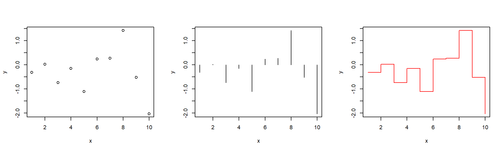
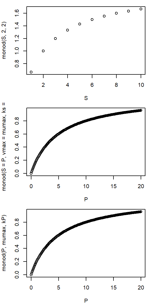
A user-defined Monod function

describes substrate dependence of biochemical turnover
widely used in biochemistry and in models
e.g. organic matter turnover in wastewater treatment

\[ v = \frac{v_{max} \cdot S}{k_S + S} \]

par(mar=c(4,4,1,1))
par(mfrow=c(3, 1))
monod <- function(S, vmax, ks) {
  vmax * S / (ks + S)
}


S <- 1:10
P <- seq(0, 20, 0.1)
kP <- 5; mumax <- 1.2;

## different ways to call the function
plot(S, monod(S, 2, 2))                # simple call
plot(P, monod(S=P, vmax=mumax, ks=kP)) # named arguments
plot(P, monod(P, mumax, kP))           # argument position

names of caller and function can be different

Seasonal Light Intensity in Dresden

\[ I_t = 997 - 816 \cos(2 \pi t / 365) + 126 \sin(2 \pi t / 365) \]

Functions as a knowledge base

put knowledge in function and use it
forget what is inside

rad <- function(t) {
  ## fill equation in
}

t <- 1:365
plot(t, rad(t), type = "l")

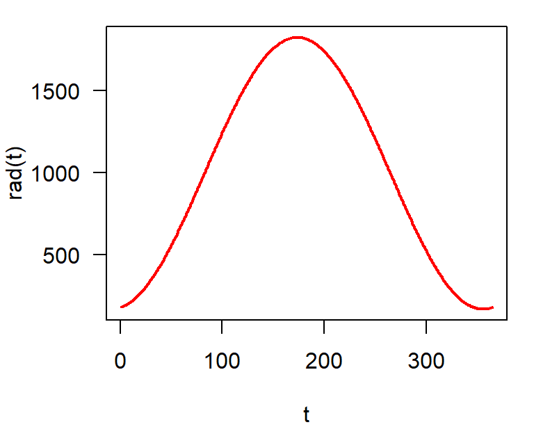
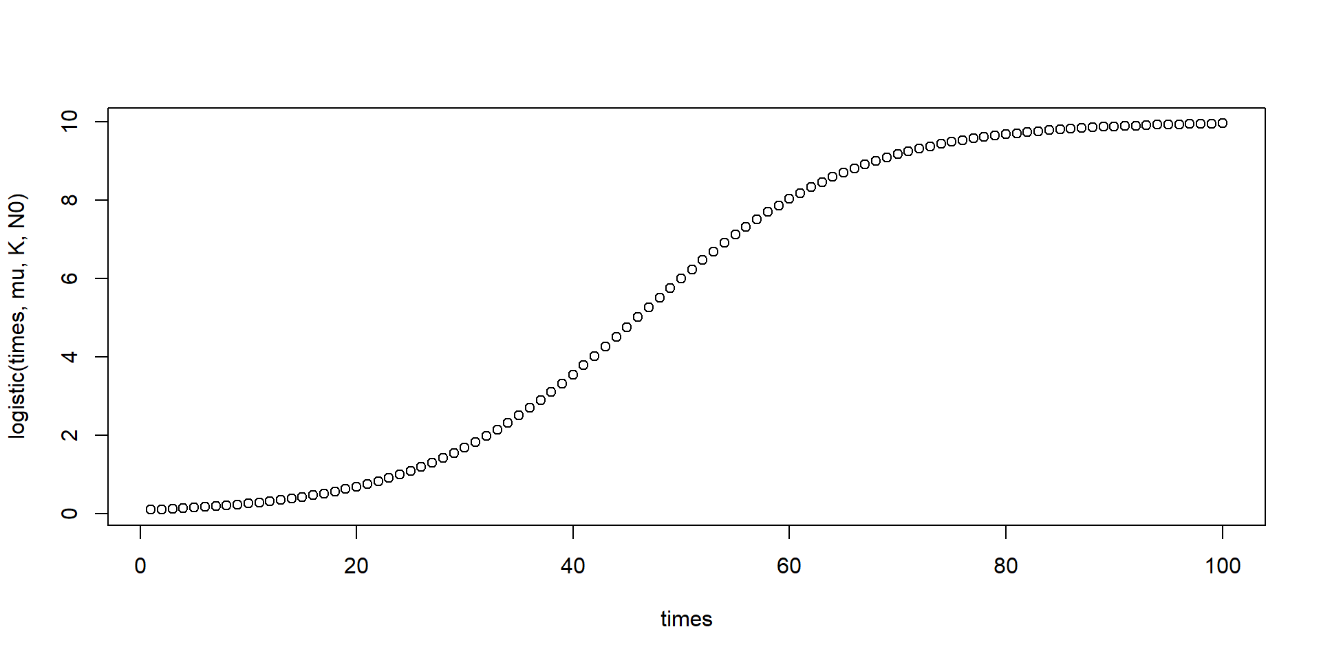
Oxygen saturation in fresh and sea water

\[ c_{O_2, 100\%} = ... ? \]

o2sat <- function(t) {
  K <- t + 273.15 # Celsius to Kelvin
  exp(-139.34411 + (157570.1/K) - (66423080/K^2) +
   (1.2438e+10/K^3) - (862194900000/K^4))
}

o2sat(20)

[1] 9.092426

A more precise formula is found in package marelac

library(marelac)
gas_O2sat(t = 20, S = 0, method = "APHA")

[1] 9.092426

consult ?gas_O2sat for citations.

Local and global variables

Variables in a function are local:

not visible from outside.
no collisions with existing variables in the calling environment

Lexical Scoping

functions can see variables of the calling function
useful for interactive work
dangerous for (exported) functions in packages
except in special cases, e.g. for functions within functions

Local and global variables II

rm(list = ls()) # remove all objects
o2sat <- function(t) {
  K <- t + 273.15 # Celsius to Kelvin
  exp(-139.34411 + (157570.1/K) - (66423080/K^2) +
   (1.2438e+10/K^3) - (862194900000/K^4))
}

o2sat(20)
K

K <- 0
o2sat(20)

Now outcomment:

# K <- t + 273.15

and try again.

Exercise

Logistic growth

The logistic growth function describes saturated growth of a population abundance \(N_t\), dependent of an initial value \(N_0\), growth rate \(r\) and carrying capacity \(K\).

\[ N_t = \frac{K N_0 e^{rt}}{K + N_0 (e^{rt}-1)} \]

logistic <- function(t, r, K, N0) {
  K*N0*exp(r*t)/(K+N0*(exp(r*t)-1))
}


mu <- 0.1; K = 10; N0 = 0.1
times <- 1:100

plot(times,
     logistic(times, mu, K, N0))

Functional response types in Ecology

Holling type I \(P = \min(k \cdot N, P_{max})\)
Holling type II \(P = \frac{\alpha N}{1 + \alpha H N}\)
Holling type III \(P = \frac{\alpha N^b}{1 + \alpha H N^b}\)

with

\(P\)	predation rate
\(N\)	abundance of prey
\(P_{max}\)	maximum predation rate
\(k\)	a constant
\(\alpha\)	attack rate
\(H\)	handling time
\(b\)	exponent \(>1\)

Write a function for each functional reponse type and plot it.
Write a universal function for all types.