library(maps)
map("world")16-Working with Maps in R
R contains many packages for working with spatial data; an overview can be found in the ‘CRAN Task View: Analysis of Spatial Data’, which can be found on the servers containing the R packages (Comprehensive R Archive Network): https://cran.r-project.org.
The packages contain, among others:
- functions for reading, writing and handling spatial data,
- import and export from and to GIS systems (ArcGIS, QGIS)
- projections, transformation of coordinate systems (package sf)
- point pattern analysis, geostatistics and spatial interpolation
- accessing and plotting maps from Google Maps and OpenStreetmap, graphing data on maps (package leaflet)
In the following, we will deal with a set of selected mapping functions. After exploring some basic methods, we will create a map showing the locations of all the people from HSE who are attending the exercise.
1 The traditional way with package maps
In the following, let’s use the packages maps for drawing geographical maps.
1.1 Plotting of Countries
Drawing a world map is as simple as:
and mapping a country can be done with:
map("world", "Germany")At time of writing, the world data base was updated in 2013. We may also consider to color the world. For this purpose, let’s use nicely designed color maps found on: http://colorbrewer2.org/
This web page allows to design color schemes and to use the codes in any software, e.g. Word or Powerpoint. For R, we can use a specific package:
library(RColorBrewer)
mycolors <- brewer.pal(12, "Set3")
map('world', col=mycolors, fill=TRUE)
Of course, we can also use other colours according to our preferences.
map('world')
map('world', "Germany", add=TRUE, col="red", fill=TRUE)
If you want to center the world to the pacific, use:
map("world",projection="rectangular",parameter=0,
  orientation=c(90,0,180), wrap=TRUE)
map("world", "Indonesia", orientation=c(90,0,180),
   col="red", fill=TRUE, add=TRUE)
Country names are in English, but they can also be derived from the 2 or three letter ISO country code, see https://countrycode.org/.
iso.expand("id")
iso.expand("idn")
1.2 Plotting cities
R contains a data base of more 40,000 world cities, including the capital cities of all countries and their population size, see ?world.cities for details.
data(world.cities)
str(world.cities)
The following plots the Capital cities:
map("world")
map.cities(capitals=1, col="red", pch=16)
The following highlights the capital cities of China (1=country capital, 2=provincial, state, or regional capital, or 3=local capital)
map(regions="China", col="lightgrey", fill=TRUE)
map.cities(country="China", minpop=1e5, col="blue", pch=16)
map.cities(country="China", capitals=1, pch=16, col="red", cex=2)
map.cities(country="China", capitals=2, pch=16, col="orange", cex=1.5)
map.cities(country="China", capitals=3, pch=16, col="green", cex=1)
And now all cities of Germany with more than 400000 inhabitants (and also the main rivers):
library("mapdata")
map("world", "Germany")
map.cities(country="Germany", capitals=1)
map.cities(country="Germany", minpop = 400000)
map.axes()
map("rivers", add=TRUE, col="blue")
The data base can also be used to retrieve the GPS coordinates of a city:
world.cities[world.cities$name=="Dresden",]
world.cities[world.cities$name=="Berlin",]
Berlin <- subset(world.cities, name=="Berlin" & country.etc == "Germany")
The circles can also represent the size of the city. Taking the square root ensures that it is the area of the circle, rather than the diameter, that is proportional to the population. Scaling the circles by 500,000 gives a reasonable size.
map("world", "Germany")
map.cities(country="Germany", pch=16, col="blue",
       cex=sqrt(world.cities$pop/5e5))
points(Berlin$long, Berlin$lat, col="red", pch=16,
       cex=sqrt(Berlin$pop/5e5))
2 A world map of course participants
2.1 A standard map
- Collect data of your home cities from all participants
- Draw a world map
- Highlight all your home cities in the world map
Use the following example of German cities > 40,0000 inhabitants as a template
cities.de <- subset(world.cities, country.etc =="Germany" & pop > 400000)
cities.demap("world", "Germany")
points(cities.de$long, cities.de$lat, pch=16, col="red")
text(cities.de$long, cities.de$lat, cities.de$name, cex=0.7, pos=1)2.2 A globe
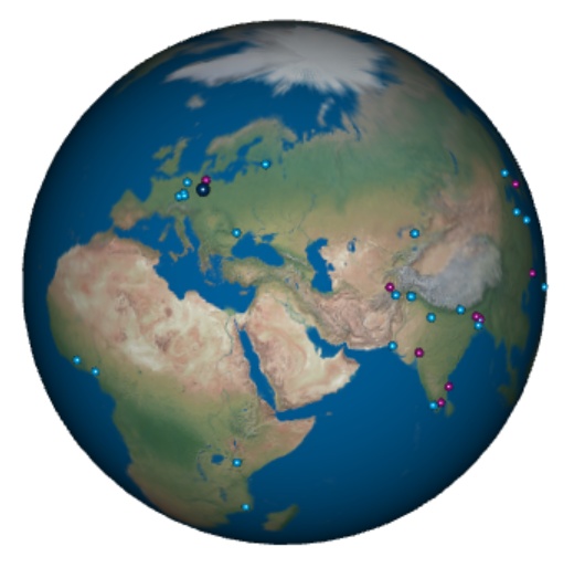
With the data collected above, it is now possible to create a web page with a globe to see how your fellow students came from. This globe can be embedded in an interactive web page. A live-example can be found here, together with the RMarkdown source code.
3 Maps with the leaflet package
Leaflet is an open source library for interactive maps. It is written in JavaScript and allows to download maps on the fly from data providers like OpenStreatmap. It can be used in R without JavaScript knowledge by employing the leaflet R-package.
An extensive documentation is found at https://rstudio.github.io/leaflet/.
The resulting image is then a web page rather than an ordinary R graphics, so it is easy to embed it in a HTML document generated by Quarto. It is also possible to embedded in PDF or Word files.
The leaflet package is compatible to pipelines in tidyverse (%>%) and to native R pipes (|>).
In the following, we set a range of coordinates for the university and add markers for two buildings. The function call then downloads the map from OpenStreetmap on the fly and adds two markers and a popup.
library(leaflet)
leaflet() |>
  addTiles() |>
  setView(lng = 13.7254, lat = 51.0282, zoom = 15) |>
  addPopups(lng = 13.7254, lat = 51.0282,
             popup = "TU Dresden") |>
  addMarkers(lng = c(13.7228, 13.73043),
             lat = c(51.02556, 51.0277),
             popup = c("APB", "CHE"),
             options = markerOptions(title=c("Computer Science Building",
                                             "Chemistry and Hydro Science"))
  )
Leaflet can also be used to plot polygons and filled areas. This is slightly more complex and will be left for you to experiment with later.
3.1 Web links and custom map symbols
Package leaflet supports custom map markers from different icon libraries, for example from https://www.glyphicons.com/. In addition, marker popup texts may also contain web links. The map below shows the central TU Dresden campus with some of the cafeterias, as well as the Drudebau, the Hydrosciences and the Computer Science buildings. Click on one of the cutlery icons to access the Mensa menu.
library(leaflet)

i_parking <- makeAwesomeIcon(icon = 'P', markerColor = 'blue',
               library='glyphicon', fontFamily="Open Sans", text="P")
i_mensa   <- makeAwesomeIcon(icon = 'cutlery', markerColor = 'red',
               library='glyphicon')
i_edu     <- makeAwesomeIcon(icon = 'education', markerColor = 'darkblue',
              library='glyphicon')
i_home    <- makeAwesomeIcon(icon = 'home', markerColor = 'darkblue',
              library='glyphicon')

lunch <- "https://www.studentenwerk-dresden.de/mensen/speiseplan/"

leaflet()|>
  addTiles()|>
  setView(lng = 13.735, lat = 51.034, zoom = 15) |>
  addAwesomeMarkers(lng = c(13.72292, 13.73067), lat = c(51.02559, 51.02804),
             popup = c("Pfitzmannbau","Chemistry/Hydrosciences"),
             icon =  i_edu) |>
  addAwesomeMarkers(
    lng = c(13.72867, 13.73868, 13.72645, 13.74902, 13.73394, 13.7293),
    lat = c(51.03146, 51.02960, 51.02708, 51.030, 51.03440, 51.03028),
    popup = c(paste0("<a href=", lunch, ">Mensa</a> Zeltschlösschen"),
              paste0("<a href=", lunch, ">Mensa</a> Siedepunkt"),
              paste0("<a href=", lunch, ">Mensa</a> Alte Mensa"),
              paste0("<a href=", lunch, ">Mensa</a> WuEins"),
              paste0("<a href=", lunch, ">Mensa</a> Reichenbachstraße"),
              paste0("<a href=", lunch, ">Mensa</a> U-Boot")),
    icon = i_mensa) |>
  addAwesomeMarkers(lng = 13.74780, lat = 51.02769,
             popup = "Hydrobiologie\nDrude-Bau", icon = i_home)
3.2 Alternative map providers
Now let’s plot a water body and annotate different sampling stations. Here we use addCircleMarkers with different colors. As an addtional option, let’s replace addTiles() with `addProviderTiles(“OpenTopoMap”) for an alternative base map:
leaflet() |>
  #addTiles() |>                         # standard OpenStreetmap
  addProviderTiles("OpenTopoMap") |>     # A topographical map
  setView(12.22, 50.535, zoom = 12) |>
  addMarkers(12.20296, 50.54397, label="littoral station") |>
  addCircleMarkers(12.195, 50.537, radius=5, color="red", label="buoy 1") |>
  addCircleMarkers(12.19, 50.542, radius=5, color="blue", opacity=1,
    label = "buoy 2")
A list of available map providers can be found at https://leaflet-extras.github.io/leaflet-providers/preview/. Some maps can be used out of the box, some others need some experimentation.
More about maps with R can be found in the package documentations and on several web pages, just use your favorite search engine.
4 Exercises
- Experiment with the leaflet map tools. Select appropriate coordinates and suitable zoom levels.
- Create maps of your favorite locations in Dresden and in your hometown, e.g. your flat, the university, or your recreational area.
- Create a postcard and with this map and send it to your friends.