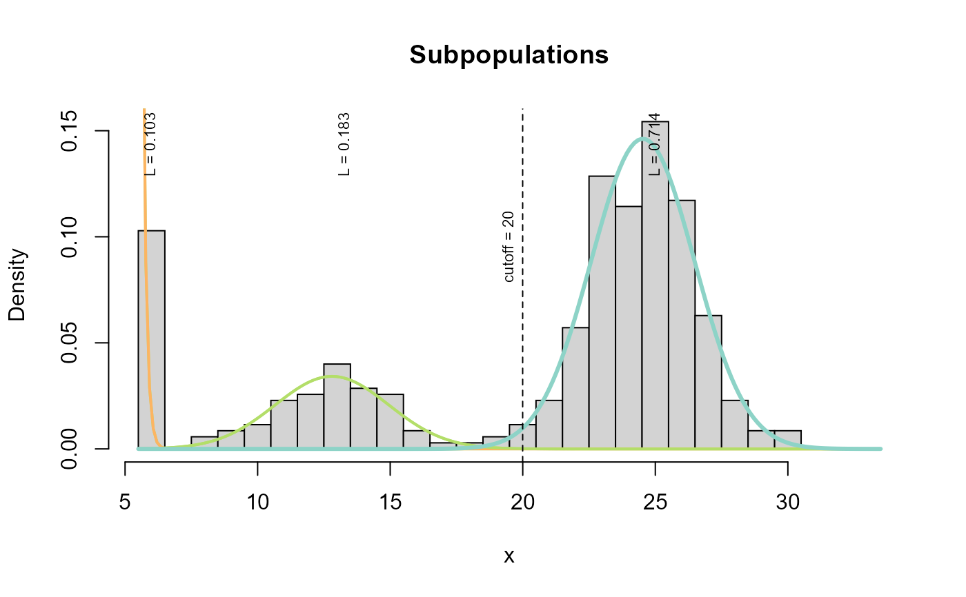
Plot Components of Mixture Distribution

mx_plot(
  obj,
  breaks,
  counts,
  disc = 0,
  ecoff.prob = 0.01,
  main = "Subpopulations",
  length.out = 200,
  ...
)

Arguments

obj	Object of class `mxObj`.
breaks	class boundaries
counts	frequency of observations
disc	disc diameter (defaults to zero)
ecoff.prob	probability threshold for the ecoff
main	main title of the plot
length.out	number of points used for plotting component densities
...	other arguments passed to `hist`

Value

ecoff value (normal quantile)

Examples


breaks <- 0:28
counts <- c(36, 0, 2, 3, 4, 8, 9, 14, 10, 9, 3, 1, 1, 2,
            4, 8, 20, 45, 40, 54, 41, 22, 8, 3, 3, 0, 0,0)

observations <- unbin(breaks[-1], counts) # upper class boundaries

(comp <- mx_guess_components(observations, bw=2/3, mincut=0.9))
#>        mean        sd         L
#> 1  1.040054 0.7032986 0.1055751
#> 2  7.805322 2.0509038 0.1775396
#> 3 19.505968 2.1153693 0.7168853

obj <- mxObj(comp, left="e")

obj2 <- mx_metafit(breaks, counts, obj)

mx_plot(obj2, breaks, counts, disc=5.5)

## simplification for fitted objects with save.data = TRUE
mx_plot(obj2, disc=5.5)