x05-Creation of Reports with Quarto
Applied Statistics – A Practical Course
Thomas Petzoldt
2026-01-28
About these slides
The slides were created with Quarto using Rstudio and R.
Use cursor keys for navigation, press O for a slide Overview
Markdown, RMarkdown and Quarto
Markdown .md
- ” … is a lightweight markup language for creating formatted text using a plain-text editor” (Wikipedia, 2022).
- Can be written with any text editor, less perfect than Latex, but much easier.
- Markdown supported by many programs and services (e.g. Github, StackOverflow, Matrix, RStudio, …)
RMarkdown .Rmd
- is an extension of markdown that can embed R code.
- superseeded by Quarto
Quarto .qmd
- is an extension of Markdown that can embed R, Python, Julia and Observable code.
- improved capabilities to create reports, slides, websites, papers, books.
Why Markdown or Quarto
Quick note taking (documentation of ideas, experiments, SOPs, …)
Documentation of statistical analyses (Quarto + R)
Clearly structured documents (outline clearly visible)
Easy literature referencing
Much easier than LaTeX
Widely used technology, useful for Stackoverflow, Github or Matrix
Software
- You can use any text editor, e.g. Notepad++, your mail client
… or even Word
- Better: use an editor with Markdown support
- RStudio
- PanWriter, a basic writing program with an almost empty screen
\(\rightarrow\) distraction free writing - Joplin, a note taking program with cloud connectivity and encryption
- many online services: Github, Gitlab, StackOverflow, Matrix
- and more
Many Markdown Programs Available, e.g. Panwriter
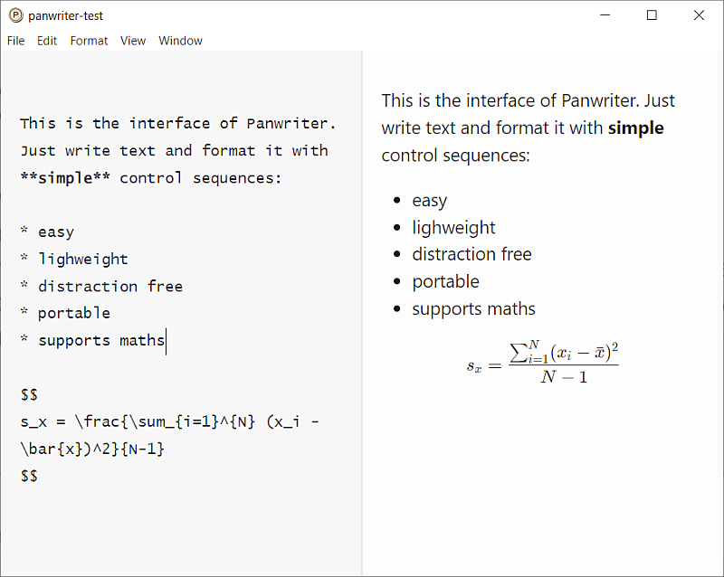
Panwriter with live preview
Let’s use RStudio. Supports Markdown and Quarto
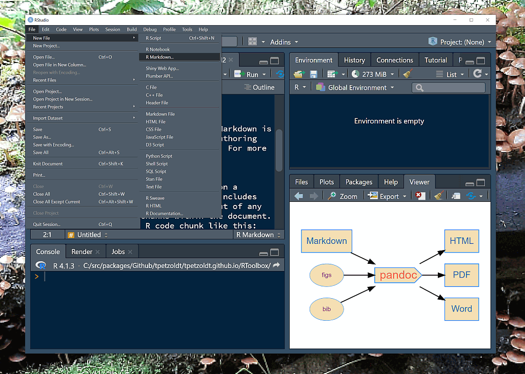
RStudio
Example
Section titles are introduced with one or several hash symbols #, ##, praragraphs with empty lines, italic and bold face are indicated with one or two starts before and after a phrase, bullet points with a leading dash - or a star *. Weblinks are automatically activated. Here an example:
    # First level

    Text can be written with any editor, that can be formatted, e.g. *slanted*, **boldface**,
    `verbatim text` weblinks: https://tu-dresden.de or bullet points:

    * point 1
    * point 2

    Section titles start with one or more hash tags


    ## Second level

    ### Third level
There are of course more formatting options, found in the docs or explained later.
YAML Header
Quarto and markdown documents can have a few special lines on top, enclosed within three dashes ---. This so called “YAML header” is used to set text settings and formatting options:
    ---
    title: "Test"
    author: "Who wrote this"
    date: '2024-11-12'
    format: html
    ---

    # First Section

    Lorem ipsum dolor sit amet, consetetur sadipscing elitr, sed diam nonumy
    eirmod tempor invidunt ut labore et dolore magna aliquyam erat.

    At vero eos et accusam et justo duo dolores et ea rebum.

    # Second Section

    Stet clita kasd gubergren, no sea takimata sanctus est Lorem ipsum
    dolor sit amet.
YAML: yet another markup language. A list format coming from the python world.
Layout and format conversion
- User can concentrate on writing, formatting is done automatically.
- Several tools exist to convert markdown to other document formats.
- One of the most popular is pandoc. It is built-in in Rstudio.
Rendering is done with the pandoc utility to convert Quarto or Markdown text to
HTML for web pages, pdf for printing, or Word for further editing.
What is Pandoc?
- Pandoc is a universal text conversion tool
- It is said to be the “swiss-army knife” to convert between formats
- Open Source licensed: GPL 2.0 resp. MIT license
- Available from: https://pandoc.org/
- … or embedded in RStudio
Exercise
- Write your first Quarto document in RStudio.
- Render it to HTML and Word
Optional without warranty
- Create PDF output
- Needs LaTeX type setting system installed
- Can be done with R’s tinytex package:
::: {.cell}

:::
… or by installing tinytex from the Terminal of RStudio
quarto install tinytexand then include format: pdf in the YAML header
title: "My document"
format: pdf
See more at: https://quarto.org/docs/output-formats/pdf-basics.html
Section Titles
Section titles can be formatted with hashtags or by underlining:
# A Section

## A subsection
or:
A Section
=========

A Subsection
------------
Automatic numbering can optionally be enabled in the YAML header:
---
title: "My document"
format:
  html:
    toc: true
    number-sections: true
---
Weblinks
Formatted weblinks
[further reading](https://rmarkdown.rstudio.com)
is then formatted as: further reading
Example
The [*Markdown Wikipedia page*](https://de.wikipedia.org/wiki/Markdown) contains examples.
The Markdown Wikipedia page contains examples.
Images
Images are similar to weblinks, but with a leading !

figure title
Verbatim Text
Verbatim text can be created with several methods:
- Inline: enclose text within single backticks
`verbatim text`\(\rightarrow\)verbatim text - Indentation by 4 spaces
- Use so-called fencing with
```before and after a tect or code block.
```
Lorem ipsum dolor sit amet, consetetur sadipscing elitr, sed diam nonumy
eirmod tempor invidunt ut labore et dolore magna aliquyam erat, sed diam
voluptua.
```
appears as:
Lorem ipsum dolor sit amet, consetetur sadipscing elitr, sed diam nonumy
eirmod tempor invidunt ut labore et dolore magna aliquyam erat, sed diam
voluptua.
Tables
Source code:
| Right | Left | Default | Center |
|------:|:-----|---------|:------:|
|    12 | 34   |   56    |   78   |
| this  | is   |   a     | table  |
HTML Output:
| Right | Left | Default | Center |
|---|---|---|---|
| 12 | 34 | 56 | 78 |
| this | is | a | table |
PDF output:
- Style similar to a scientific paper.
Bigger or more complex tables: create the table in Excel or LibreOffice and add markdown formatting, or use R and kable to create the table from data.
Citations
Create database file in .bib-format, e.g. references.bib
- can be exported from Zotero
- put bibliography file to the document folder
Use @bib_key-syntax
- textual citation: American Psychological Association (2020b) \(\leftarrow\)
@APA2020b - parenthetical citation: (American Psychological Association, 2020a) \(\leftarrow\)
[@APA2020a]
Declare bibliography in YAML header
bibliography: references.bib
csl: apa- and optionally a
.csl-style e.g.apa.csl, that is copied to the folder of the document - csl styles can be found here: https://citationstyles.org/authors/
Mathematical Formulae
Markdown and Quarto support a subset of the LaTeX formula syntax
Inline formula
$s_x = \frac{\sum_{i=1}^{N} (x_i - \bar{x})^2}{N-1}$ \(\quad \rightarrow \qquad s_x = \frac{\sum_{i=1}^{N} (x_i - \bar{x})^2}{N-1}\)
#### Display formula
$$s_x = \frac{\sum_{i=1}^{N} (x_i - \bar{x})^2}{N-1}$$\[s_x = \frac{\sum_{i=1}^{N} (x_i - \bar{x})^2}{N-1}\]
Mathematical symbols
\(\rightarrow, \le, \approx, \mu, \delta, \int, \infty, \mathrm{m^3s^{-1}}\)
$\rightarrow, \le, \approx, \mu, \delta, \int, \infty, \mathrm{m^3s^{-1}}$
More maths and chemistry
\[\begin{align} \frac{dX_1}{dt} &= k_1 \cdot X_1 - k_2 X_1 X_2 \\ \frac{dX_2}{dt} &= - k_4 \cdot X_2 + k_3 X_1 X_2 \\ \end{align}\]
\begin{align}
\frac{dX_1}{dt} &=  k_1 \cdot X_1 -  k_2 X_1 X_2 \\
\frac{dX_2}{dt} &=  k_3 X_1 X_2 - k_4 \cdot X_2 \\
\end{align}
\[\rm 6CO_2 + 6H_2O \rightarrow C_6H_{12}O_6 + 6O_2 \quad \Delta H^0 = +2870 kJ mol^{-1}\]
$$\rm 6CO_2 + 6H_2O \rightarrow C_6H_{12}O_6 + 6O_2 \quad \Delta H^0 = +2870 kJ mol^{-1}$$Embedding of R in Quarto Documents
Create a Quarto template from the File menu in RStudio. Then make your changes and click the Render button. Then, a document will be generated that includes both content as well as the output of any embedded R code chunks.
Then embed your own R code chunks like this:
```{r iris_summary}
summary(iris)
```
To show both, the code and the output
  Sepal.Length    Sepal.Width     Petal.Length    Petal.Width
 Min.   :4.300   Min.   :2.000   Min.   :1.000   Min.   :0.100
 1st Qu.:5.100   1st Qu.:2.800   1st Qu.:1.600   1st Qu.:0.300
 Median :5.800   Median :3.000   Median :4.350   Median :1.300
 Mean   :5.843   Mean   :3.057   Mean   :3.758   Mean   :1.199
 3rd Qu.:6.400   3rd Qu.:3.300   3rd Qu.:5.100   3rd Qu.:1.800
 Max.   :7.900   Max.   :4.400   Max.   :6.900   Max.   :2.500
       Species
 setosa    :50
 versicolor:50
 virginica :50
Tables from R
If you want to include real tables, you can create the table in R and then format it with knitr::kable
```{r iris_table}
knitr::kable(iris[1:4, ])
```| Sepal.Length | Sepal.Width | Petal.Length | Petal.Width | Species |
|---|---|---|---|---|
| 5.1 | 3.5 | 1.4 | 0.2 | setosa |
| 4.9 | 3.0 | 1.4 | 0.2 | setosa |
| 4.7 | 3.2 | 1.3 | 0.2 | setosa |
| 4.6 | 3.1 | 1.5 | 0.2 | setosa |
The kable function has several functions for configuring table layout, see kable help page for details.
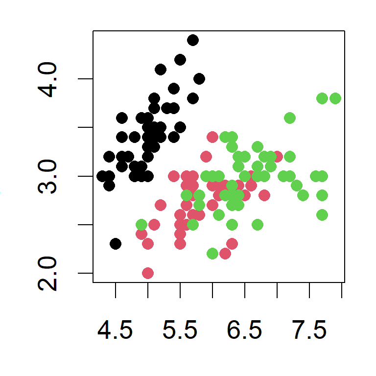
Include Plots
You can also embed plots, for example:
```{r iris_sepal}
plot(Sepal.Width ~ Sepal.Length, data=iris, pch=16, col=Species)
```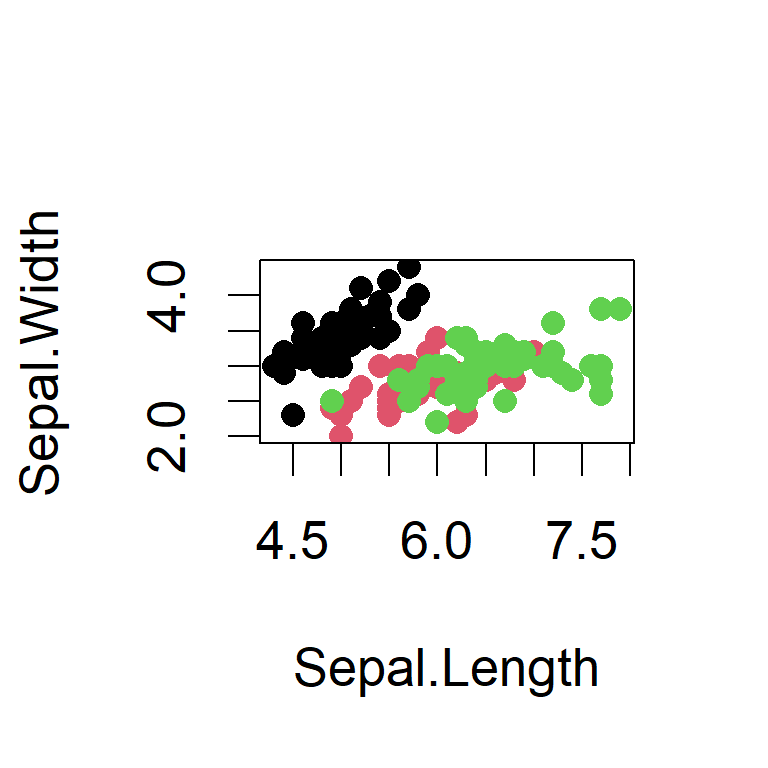
Suppress Code
The code chunks can be modified with additional options. In the following example the figure size is adjusted and an option echo = FALSE was added to prevent printing of the R code that generated the plot.
```{r iris_sepal3, fig.width=3, fig.height=3, echo=FALSE}
plot(Sepal.Width ~ Sepal.Length, data=iris, pch=16, col=Species)
```
Shows the plot without the code:
Flowcharts and graphs
… can be created with the DiagrammeR package that supports the graphviz language.
R code of the flowchart
library("DiagrammeR")
grViz("digraph pandoc {
         graph [rankdir = LR]
           node [shape = 'box']
                Markdown HTML PDF Word
           node [shape = cds]
             pandoc
           node [shape = oval]
             figs bib
           edge [penwidth=2]
             Markdown -> pandoc
             {figs bib} -> {pandoc}
             pandoc -> {HTML PDF Word}
}")
More at: https://graphviz.org/
Further reading
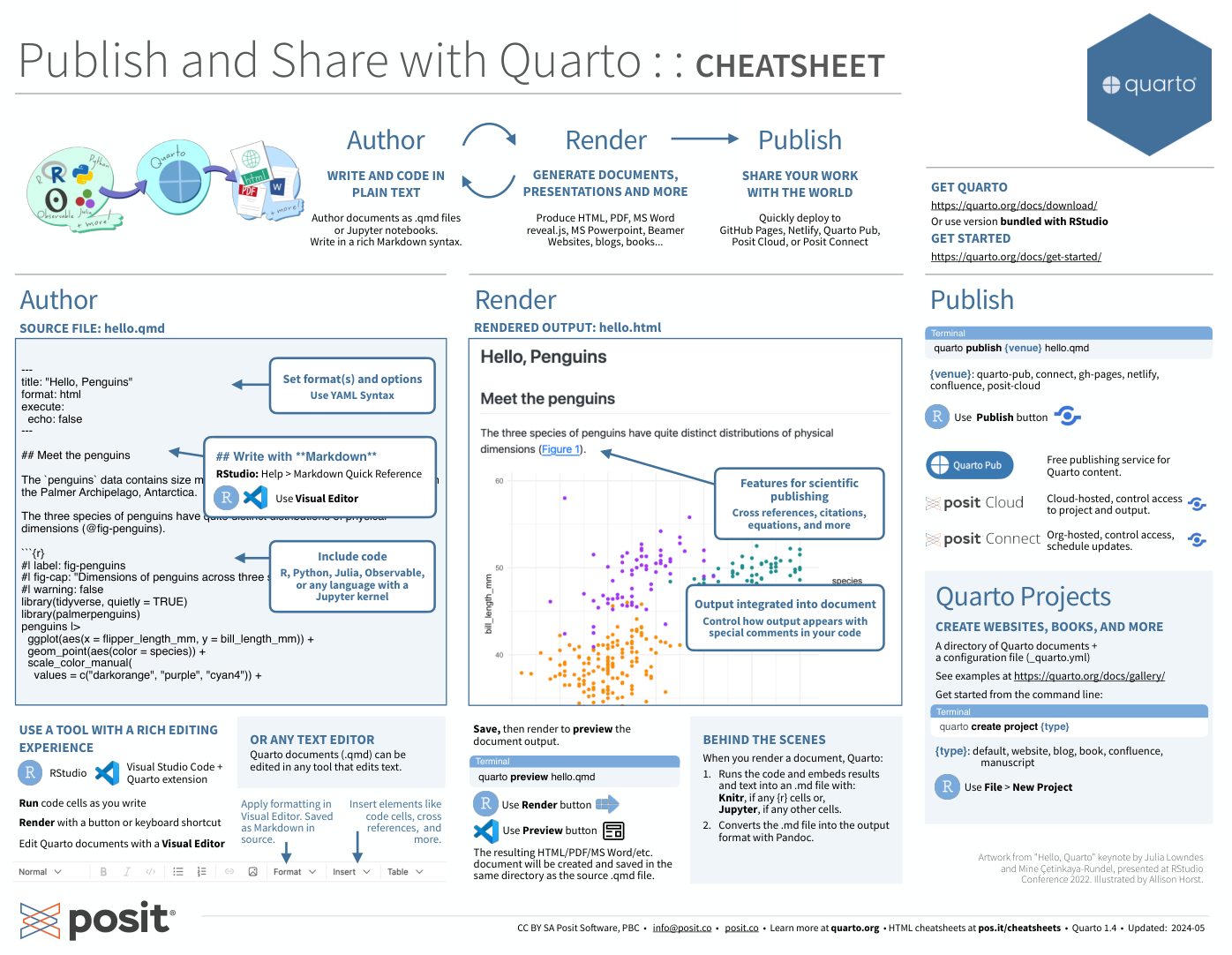
\(\rightarrow\) Quarto cheat sheet
For more details, see https://quarto.org and R Core Team (2024)“, RStudio Team (2021), Xie (2015) and The Quarto Dev Team (2024).
Thesis templates for Hydrobiology students at TU Dresden: https://github.com/tpetzoldt/hyb-tud-thesis-starterkit in Word, Latex and Quarto format. It may also be useful for you.
References
American Psychological Association. (2020a). Concise guide to APA style: The official APA style guide for students (7th ed.).
American Psychological Association. (2020b). Publication manual of the American Psychological Association: The official guide to APA style. (7th ed.).
R Core Team. (2024). R: A language and environment for statistical computing. R Foundation for Statistical Computing. https://www.R-project.org/
RStudio Team. (2021). RStudio: Integrated development environment for R. RStudio, PBC. http://www.rstudio.com/
The Quarto Dev Team. (2024). Quarto. An open-source scientific and technical publishing system. https://quarto.org
Wikipedia. (2022). Markdown. Wikipedia. https://en.wikipedia.org/w/index.php?title=Markdown&oldid=1079645429
Xie, Y. (2015). Dynamic documents with R and knitr (2nd ed.). Chapman; Hall/CRC. https://yihui.org/knitr/