Square root transformation
Wisconsin double standardization
Run 0 stress 0.1102424
Run 1 stress 0.1102424
... Procrustes: rmse 3.987625e-06  max resid 1.030191e-05
... Similar to previous best
Run 2 stress 0.1105543
... Procrustes: rmse 0.02428622  max resid 0.07215017
Run 3 stress 0.2192927
Run 4 stress 0.1102424
... Procrustes: rmse 6.092371e-06  max resid 1.658189e-05
... Similar to previous best
Run 5 stress 0.1105543
... Procrustes: rmse 0.02427623  max resid 0.07211644
Run 6 stress 0.1727865
Run 7 stress 0.1105544
... Procrustes: rmse 0.02432214  max resid 0.07227173
Run 8 stress 0.1105543
... Procrustes: rmse 0.02424285  max resid 0.07200517
Run 9 stress 0.1105543
... Procrustes: rmse 0.02420525  max resid 0.07187834
Run 10 stress 0.1105543
... Procrustes: rmse 0.02420887  max resid 0.07190017
Run 11 stress 0.2192927
Run 12 stress 0.1102424
... Procrustes: rmse 2.66011e-06  max resid 4.7284e-06
... Similar to previous best
Run 13 stress 0.1736877
Run 14 stress 0.1105543
... Procrustes: rmse 0.02423465  max resid 0.0719766
Run 15 stress 0.2680828
Run 16 stress 0.1102424
... Procrustes: rmse 5.006839e-06  max resid 1.296036e-05
... Similar to previous best
Run 17 stress 0.1102424
... Procrustes: rmse 6.788124e-06  max resid 1.892755e-05
... Similar to previous best
Run 18 stress 0.1102424
... Procrustes: rmse 8.597821e-06  max resid 2.439281e-05
... Similar to previous best
Run 19 stress 0.1102424
... Procrustes: rmse 2.269264e-06  max resid 5.374392e-06
... Similar to previous best
Run 20 stress 0.2435577
*** Best solution repeated 7 times
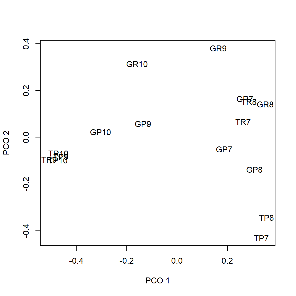
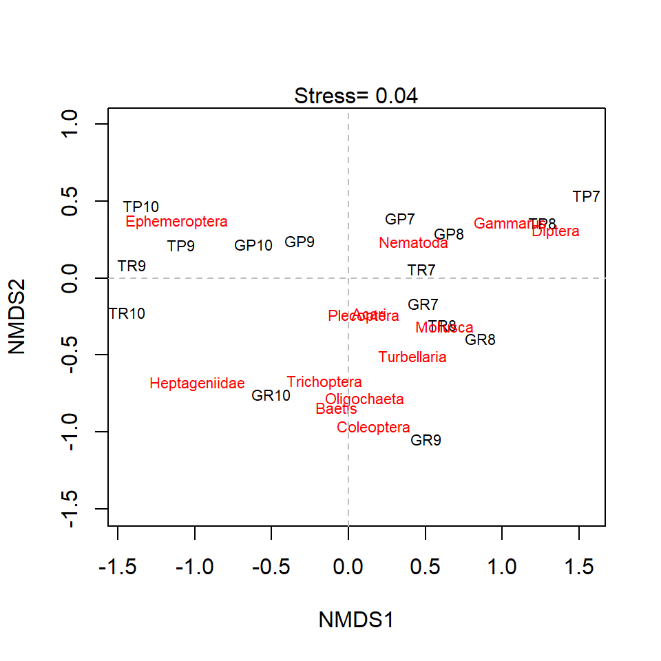
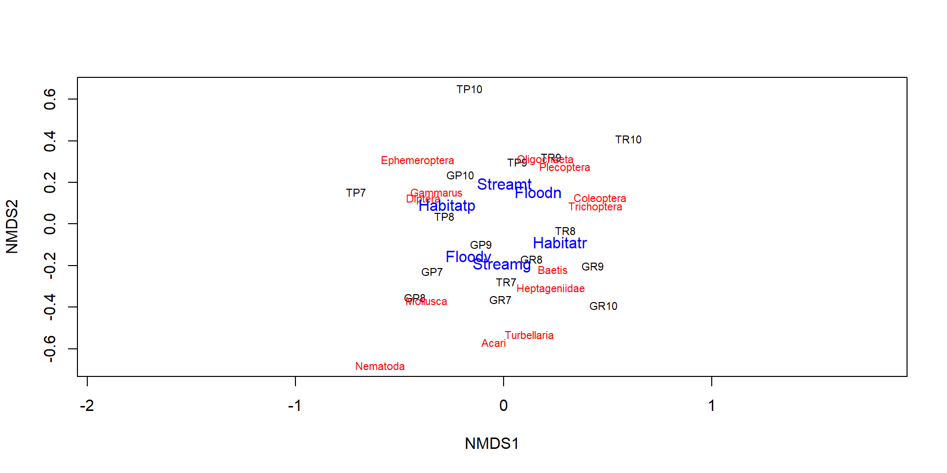
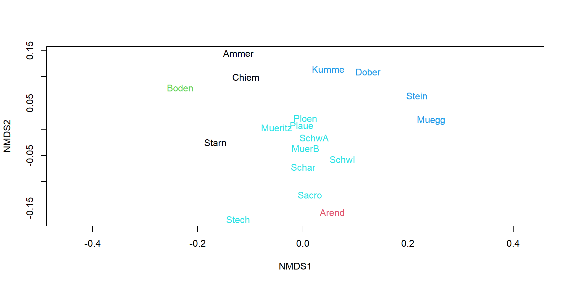
Results of the NMDS
ord
Call:
metaMDS(comm = bio)
global Multidimensional Scaling using monoMDS
Data: wisconsin(sqrt(bio))
Distance: bray
Dimensions: 2
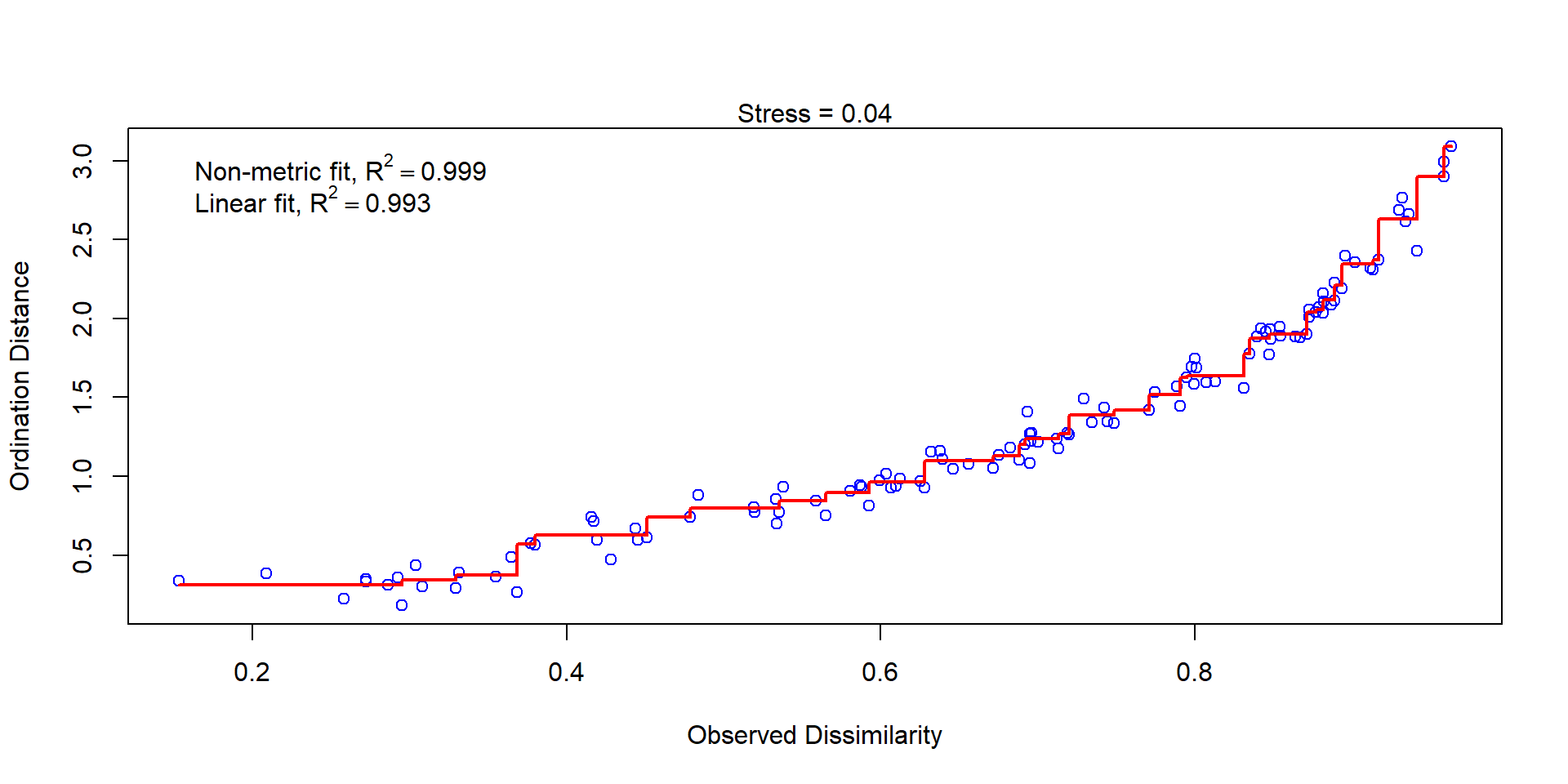
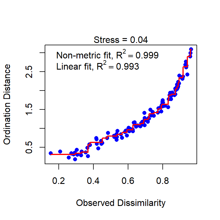
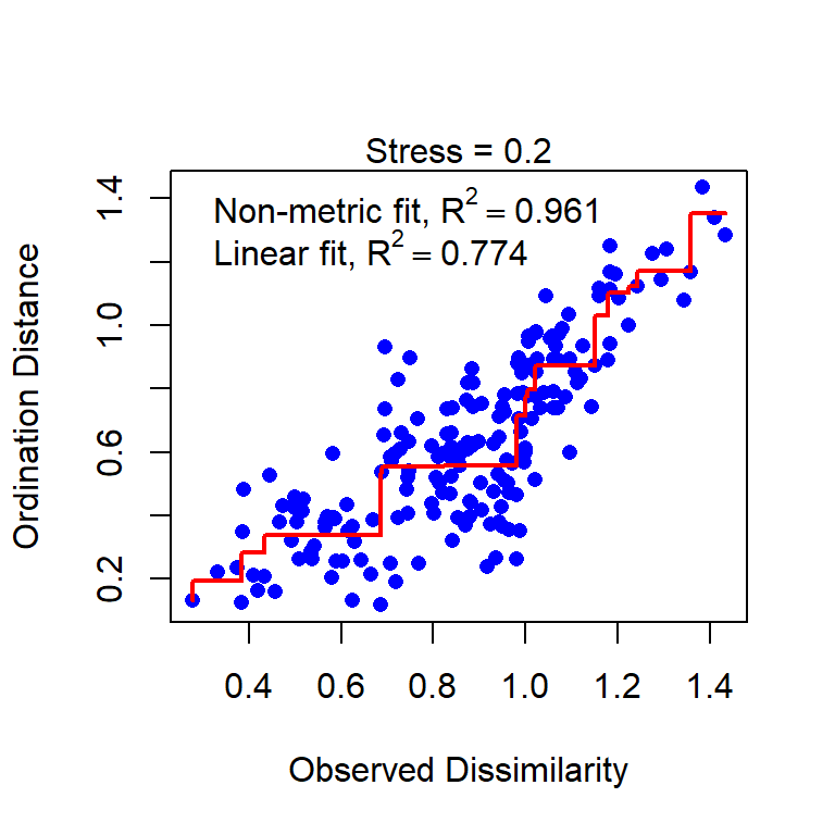
Stress: 0.1102424
Stress type 1, weak ties
Best solution was repeated 7 times in 20 tries
The best solution was from try 0 (metric scaling or null solution)
Scaling: centring, PC rotation, halfchange scaling
Species: expanded scores based on 'wisconsin(sqrt(bio))'
metaMDS runs a series of NMDS trials and outputs the best
makes automatic decisions about transformation, distance and scaling
Recommendation
specify distance, scaling and transformation explicitly
consider to increase try and trymax for big and/or difficult data sets, e.g.:
ord <-metaMDS(bio, distance="bray", autotransform=FALSE, try=40)
Pattern of stairs not important (at least not for now)
The \(R^2\) values are always big, ignore or at least don’t overinterpret it.
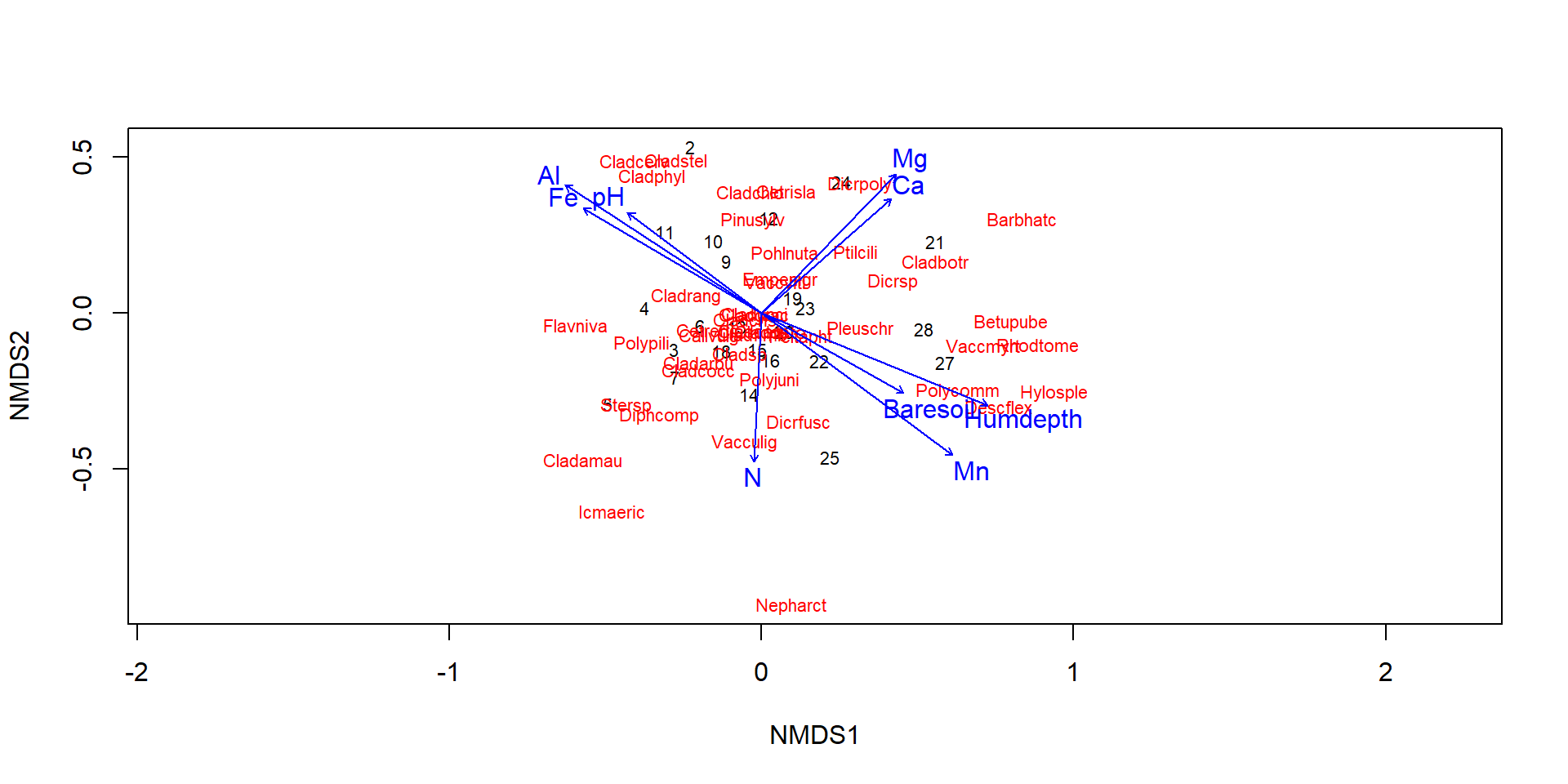
Environmental fitting
ord <-metaMDS(bio, trace =FALSE) # trace: show or suppress intermediate outputef <-envfit(ord, env, permu =1000)plot(ord, type ="t")plot(ef, p.max =0.1)
Plots arrows if explanation variables are metric.
Shows only centroids for ordinal explanation variables.
Data from Väre et al. (1995) about influence of reindeer grazin gon understorey vegetation in Pinus sylvestris forests in eastern Fennoscandia.
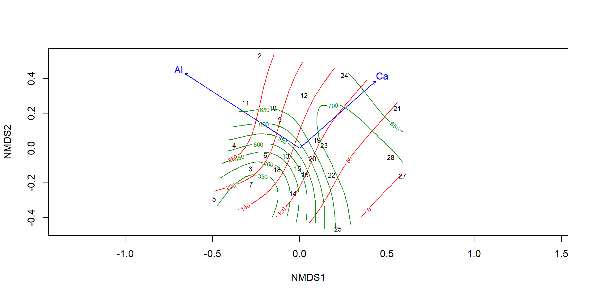
Surface fitting
ef <-envfit(mds ~ Al + Ca, varechem, permu =1000)plot(mds, display ="sites", type ="text")plot(ef)with(varechem, ordisurf(mds, Al, add =TRUE))with(varechem, ordisurf(mds, Ca, add =TRUE, col ="green4"))
Pros and cons of the methods discussed so far
PCA (and also CCA)
(+) easy to understand, quick and reproducible
(+) no non-linear distortion
(–) but: horseshoe effect possible
(–) information is often still in a “higher dimension”
(–) Euclidean distance poorly suited for species lists
NMDS
(+) any distance measure can be used
(+) better mapping on low dimensions
(–) bias
(–) numerical effort, iterative method, local minima
(–) one-matrix method (no separate matrices for species and environmental factors)
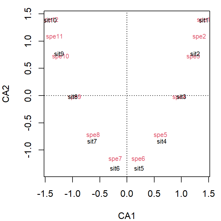
Problems of CA (and PCA)
arc (CA) or horseshoe effect (PCA)
1
1
1
0
0
0
0
0
0
0
0
0
0
1
1
1
0
0
0
0
0
0
0
0
0
0
1
1
1
0
0
0
0
0
0
0
0
0
0
1
1
1
0
0
0
0
0
0
0
0
0
0
1
1
1
0
0
0
0
0
0
0
0
0
0
1
1
1
0
0
0
0
0
0
0
0
0
0
1
1
1
0
0
0
0
0
0
0
0
0
0
1
1
1
0
0
0
0
0
0
0
0
0
0
1
1
1
0
0
0
0
0
0
0
0
0
0
1
1
1
Workaround
detrended correspondence analysis (DCA) used in the past, not anymore recommended (except you know what you do)
better: NMDS or a “constrained” (2-matrix) method, e.g. CCA, RDA, dbRDA)
Two matrix methods
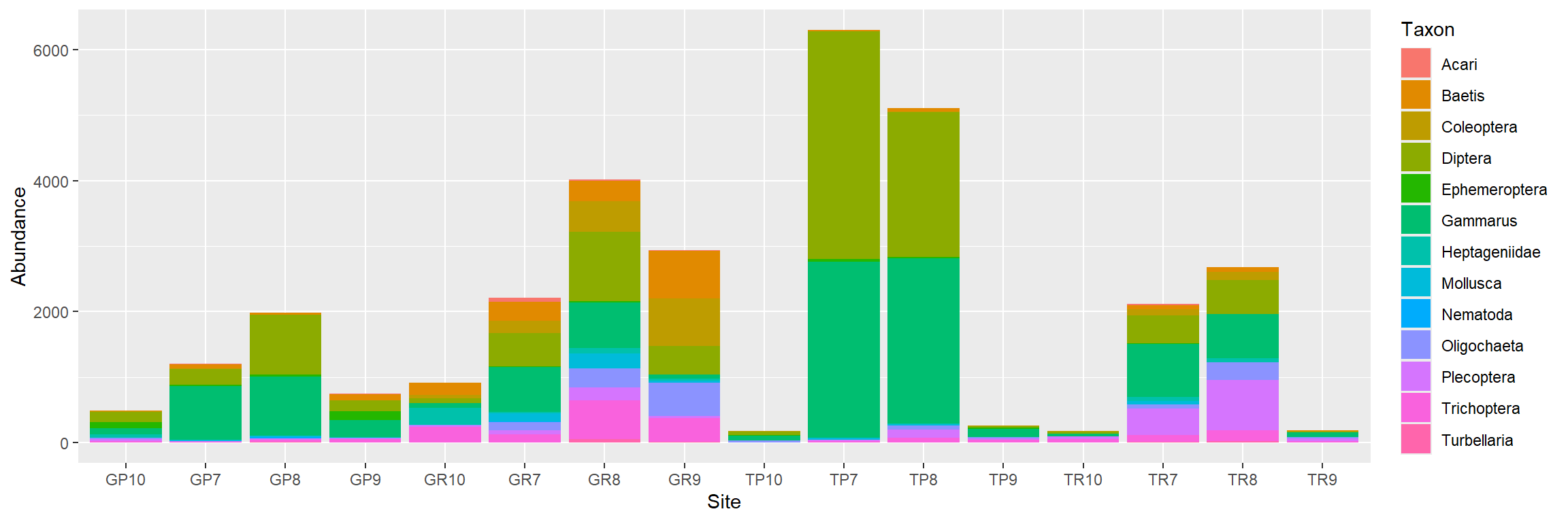
taxa matrix (bio): dependend variables, in ecology typically species
environmental matrix (env): explanation variables, also called constraints
Single matrix methods: ordination of species table alone, environmental variables considered afterwards
Two matrix methods: Species table and environmental variables treated simultanaeously
Many to many relationship
\[\mathbf{Y} = f(\mathbf{X})\]
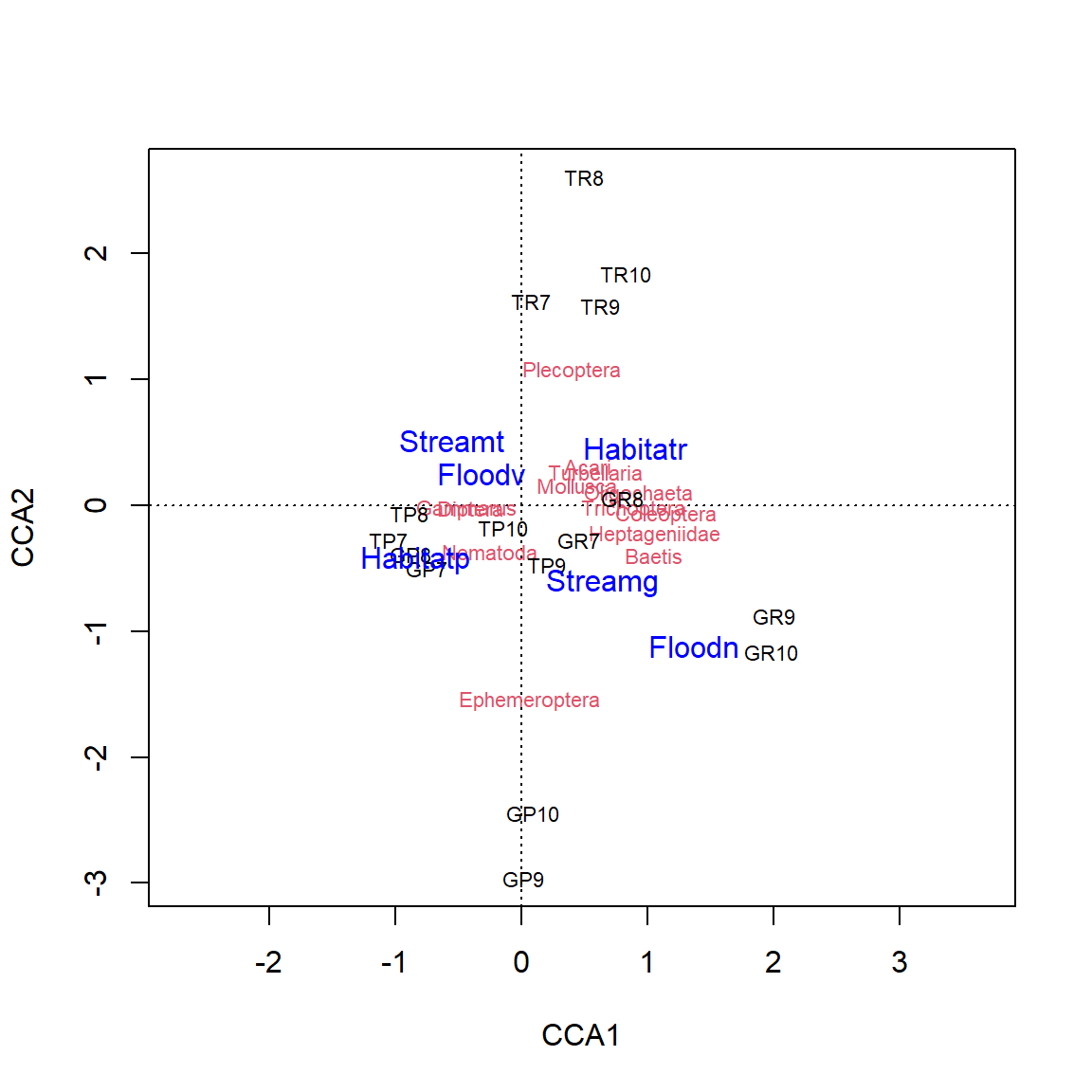
CCA: Canonical Correspondence Analysis
Example Gauernitzbach-data
ord <-cca(bio ~ ., data = env) # ~ . is an abbreviation for all variables in envord
inertia measures error and information (similar to variance)
allows separation of variability into information and error
in case of CCA it is \(\chi^2\) distance, in case of RDA it is variance
in the example
61% is explained by the constrained axes Habitat, Stream and Flood
39% is not explained by the provided environmental variables
Triplot
plot(ord)
Important
The plot shows only the part of variation that is explained by the constraints.
It the number of constraints is high compared to the number of observations, the ordination shows again the full variation, i.e. becomes unconstrained.
Interpretation of the CCA
triplot with observations, species and environmental factors, note different scaling!
distance from the origin: \(\chi^2\)
species in the middle: either “average species” or poorly explained species
species at the very edge: attention, often rare species
orthogonal angle of species on connecting line origin - centroid of environmental factor
Statistical significance: ANOVA like permutation test
anova(ord, by ="terms")
Permutation test for cca under reduced model
Terms added sequentially (first to last)
Permutation: free
Number of permutations: 999

Model: cca(formula = bio ~ Habitat + Stream + Flood, data = env)
         Df ChiSquare       F Pr(>F)
Habitat   1   0.31255 11.0671  0.001 ***
Stream    1   0.10766  3.8123  0.078 .
Flood     1   0.10081  3.5696  0.071 .
Residual 12   0.33889
---
Signif. codes:  0 '***' 0.001 '**' 0.01 '*' 0.05 '.' 0.1 ' ' 1
anova(ord, by="axis") tests significance of the CCA axes and anova(ord, by="margin") the marginal effects of the terms.
Permutation test for adonis under reduced model
Permutation: free
Number of permutations: 999

adonis2(formula = bio ~ Habitat * Stream * Flood, data = env, method = "bray")
         Df SumOfSqs      R2      F Pr(>F)
Model     7   3.2227 0.87112 7.7251  0.001 ***
Residual  8   0.4768 0.12888
Total    15   3.6994 1.00000
---
Signif. codes:  0 '***' 0.001 '**' 0.01 '*' 0.05 '.' 0.1 ' ' 1
Analysis of variance using distance matrices, uses a permutation test with pseudo-F ratios.
Not directly related to CCA, RDA etc.
Can use all dissimilarity measures from the vegdistfunction.
More powerful that the permutest-ANOVA, as it can handle interaction effects.
RDA and dbRDA
RDA: redundancy analysis
is the two-matrix extension of the PCA
uses Euclidean distance for the dependent variables
very useful, if the dependent matrix (“bio”) contains physical and chemical variables, e.g. temperature, nutrients, or aggregated biological data like total biomass or chlorophyll and not abundances of different species
So the inertia is splitted in three components, Conditional (the covariates), Constrained (flood) and Unconstrained.
The plot shows then the effect of the flood more clearly.
Which ordination method to start with?
Multivariate statistics is a very broad field. Experience shows that it can become quite complex and challenging, but also that it is relatively easy to start with it.
My personal recommendation
Start with PCA if working with physical, chemical and hydromorphological data. It often also works well with aggregated biomass data.
Use RDA if you have additional explanation variables (two-matrix method)
Start with NMDS if working with abundance data of species (taxa lists)
Use NMDS with envfit to explore influence of explanation variables on the ordination.
use CCA, dbRDA or PCoA to get more quantitative results, compared to NMDS.
Cluster Analysis
Overview
Cluster analysis aims to group data sets in clusters
Hierarchical clustering
build a dendrogram (a tree of grouping)
agglomerative methods
divisive methods
Different agglomeration methods
define how distance is measured between clusters
Nonhierarchical clustering
split into a given number of groups
usually no dendrogram
iterative methods
e.g. k-means, k-centroids
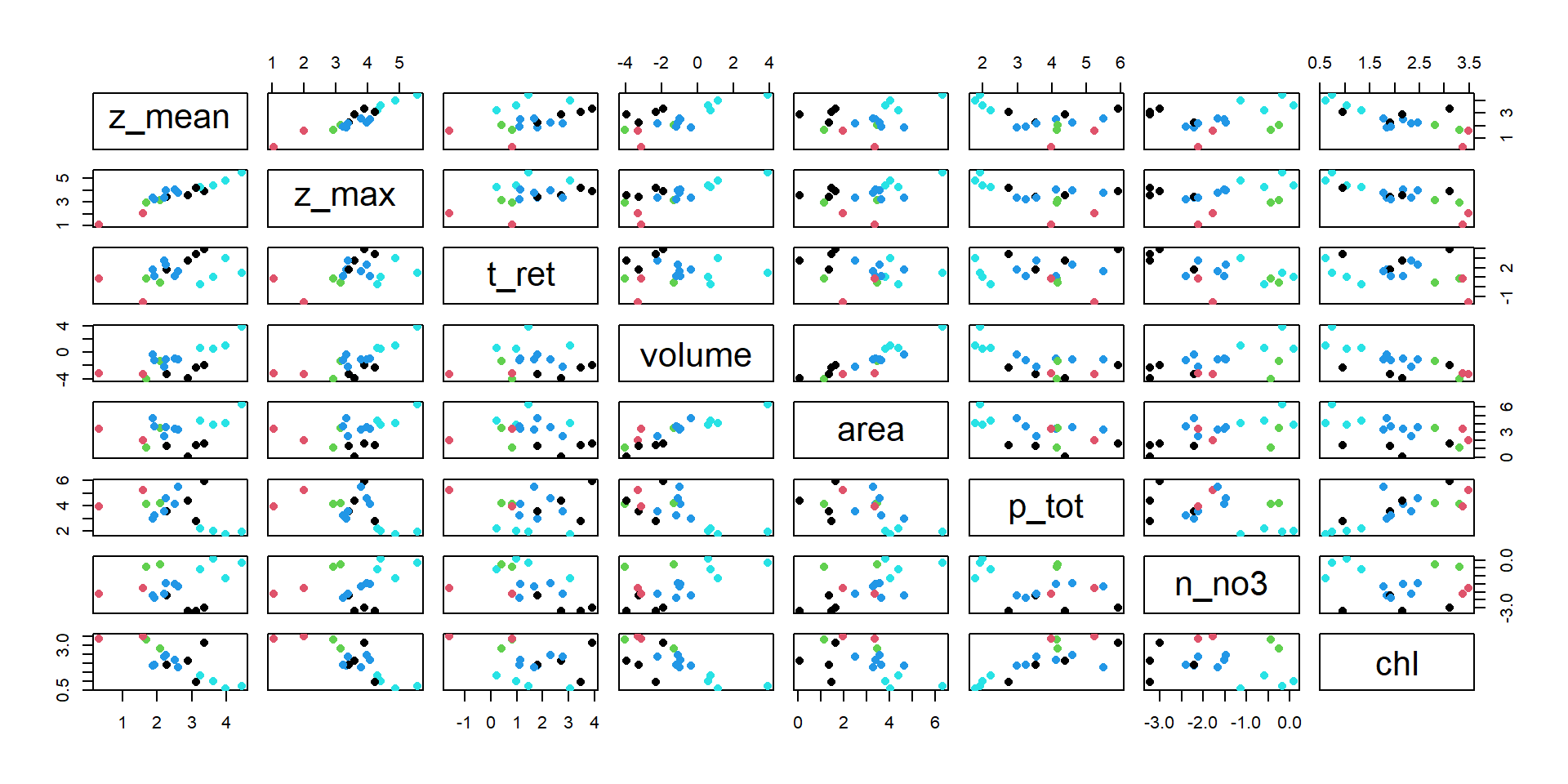
The UBA lake data set again
z_mean
z_max
t_ret
volume
area
p_tot
n_no3
chl
Ammer
37.60
81.1
2.70
1.75000
46.600
7.3
1.09
2.80
Arend
28.60
48.7
50.00
0.14700
5.140
375.0
0.05
22.30
Boden
85.00
254.0
4.20
48.52150
571.500
6.9
0.84
2.10
Chiem
25.60
73.4
1.26
2.04800
79.900
9.2
0.55
3.80
Dober
5.40
18.8
2.30
0.01690
3.120
63.9
0.64
27.30
Muegg
4.85
7.5
0.20
0.03500
7.200
189.9
0.17
32.90
Ploen
12.40
58.0
3.10
0.37200
29.970
62.3
0.22
8.80
Kumme
8.10
23.3
1.50
0.26300
32.500
65.3
0.78
16.60
Mueritz
6.50
28.1
6.00
0.68000
105.300
19.7
0.11
6.30
MuerB
9.80
30.3
6.00
0.03800
3.910
34.2
0.11
6.70
Plaue
6.80
25.5
3.00
0.30000
38.400
26.0
0.09
6.80
Sacro
18.01
36.0
15.00
0.01930
1.072
79.8
0.04
8.60
Schar
9.00
29.5
16.00
0.10823
12.090
35.3
0.12
10.40
SchwA
9.40
52.4
10.00
0.33100
35.200
100.0
0.23
11.70
SchwI
13.50
44.6
5.30
0.35600
26.400
246.5
0.19
5.86
Starn
53.20
127.8
21.00
2.99900
56.400
5.9
0.32
1.84
Stech
22.80
68.0
32.00
0.09700
4.250
15.8
0.04
2.60
Stein
1.35
2.9
2.30
0.04200
29.100
53.3
0.12
29.00
Cluster analysis
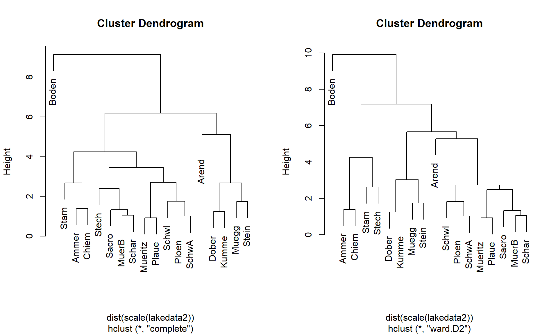
par(mfrow=c(1,2))hc <-hclust(dist(scale(lakedata2)), method="complete") # the defaultplot(hc)hc2 <-hclust(dist(scale(lakedata2)), method="ward.D2")plot(hc2)
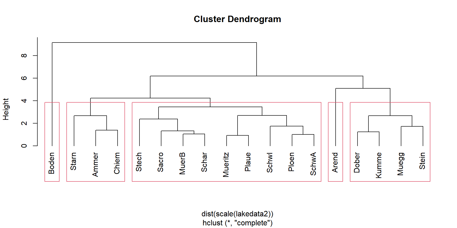
Identification of clusters in the tree
plot(hc, hang =-1) # -1: extend vertical lines to the bottomrect.hclust(hc, 5)
grp <-cutree(hc, 5)# grp # can be used to show the groups
Väre, H., Ohtonen, R., & Oksanen, J. (1995). Effects of reindeer grazing on understorey vegetation in dry Pinus sylvestris forests. Journal of Vegetation Science, 6(4), 523–530. https://doi.org/10.2307/3236351
Winkelmann, C., Hellmann, C., Worischka, S., Petzoldt, T., & Benndorf, J. (2011). Fish predation affects the structure of a benthic community. Freshwater Biology, 56(6), 1030–1046. https://doi.org/10.1111/j.1365-2427.2010.02543.x