11-Multivariate methods I

Applied Statistics – A Practical Course

Thomas Petzoldt

2025-09-16

Data sets and terms of use

1. The “UBA-lakes” data set originates from the public data repository of the German Umweltbundesamt (Umweltbundesamt, 2021). The data set provided can be used freely according to the terms and conditions published at the UBA web site, that refer to § 12a EGovG with respect of the data, and to the Creative Commons CC-BY ND International License 4.0 with respect to other objects directly created by UBA.

2. The “gauernitz” data set contains simplified teaching versions from research data, of the study from Winkelmann et al. (2011)

3. The document itself, the codes and the ebedded images are own work and can be shared according to CC BY 4.0.

An introductory example

Correlation between all variables?

library("readxl") # read Excel files directly
lakes <- as.data.frame(
  read_excel("../data/uba/3_tab_kenndaten-ausgew-seen-d_2021-04-08.xlsx", sheet="Tabelle1", skip=3)
)
names(lakes) <- c("name", "state", "drainage", "population", "altitude", 
                  "z_mean", "z_max", "t_ret", "volume", "area", "shore_length", 
                  "shore_devel", "drain_ratio", "wfd_type")
str(lakes)

'data.frame':   56 obs. of  14 variables:
 $ name        : chr  "Ammersee" "Arendsee" "Bleilochtalsperre" "Bodensee" ...
 $ state       : chr  "BY" "ST" "TH" "BW" ...
 $ drainage    : num  993 29.8 1239.9 11477 28.2 ...
 $ population  : num  114900 3200 180000 1400000 28 ...
 $ altitude    : num  532.9 22.8 404 395.4 13.1 ...
 $ z_mean      : num  37.6 28.6 23.3 85 2.4 ...
 $ z_max       : num  81.1 48.7 55 254 4.8 58.3 32.5 73.4 1.7 18.8 ...
 $ t_ret       : num  2.7 50 0.526 4.2 1.9 16.3 NA 1.26 0.1 2.3 ...
 $ volume      : num  1.75 0.147 0.215 48.522 0.009 ...
 $ area        : num  46.6 5.14 9.2 571.5 3.9 ...
 $ shore_length: num  43 9 NA 273 10.4 13.7 17.5 64 7.5 10.1 ...
 $ shore_devel : num  1.78 1.12 NA 2.26 1.48 2.09 1.64 2.02 2.22 1.6 ...
 $ drain_ratio : num  20.3 5.8 NA 21.9 7.2 ...
 $ wfd_type    : chr  "Typ 4" "Typ 13" "Typ 5" "Typ 4" ...

• names(lakes) replaces the original German column names by abbreviated English abbreviations

Create pairwise scatter plots for all variables?

plot(lakes)

Create pairwise scatter plots for all variables?

• not a good idea, 14 variables would produce 182 (or 91) plots

• can lead to “statistical fishing”

• we need methods to extract the main information with a small number of plots

The multivariate approach

Work with the complete original variables directly

\(\rightarrow\) Multivariate statistics

• dependent variables + explanation variables optional
• analyze distance and location in multidimensional space
• find way to vizualize relationship in lower dimensions

For comparison

• univariate: 1 variable
• bivariate: 1 dependent, 1 independent variable
• multiple: 1 dependent, >1 independent variables

Two approches of multivariate statistics

Ordination

• dimension reduction
• relate observations and variables

Cluster analysis

• distance and similarity
• identification of groups

Basic concepts

Similarity and correlation

• distance and similarity:
  \(\rightarrow\) How different or similar are the observations?
• correlation and covariance:
  \(\rightarrow\) Are variables interdependent?
• dimension reduction:
  \(\rightarrow\) Try to show essential parts of information on a lower number of dimensions.
• cluster analysis:
  \(\rightarrow\) Show which observations are closely together.
• ordination:
  \(\rightarrow\) Plot data at lower dimensions, similar observations closely together.

The UBA-lakes example

A data set from German lakes

GPS data from Wikipedia and Google Maps, map from https://www.openstreetmap.org/

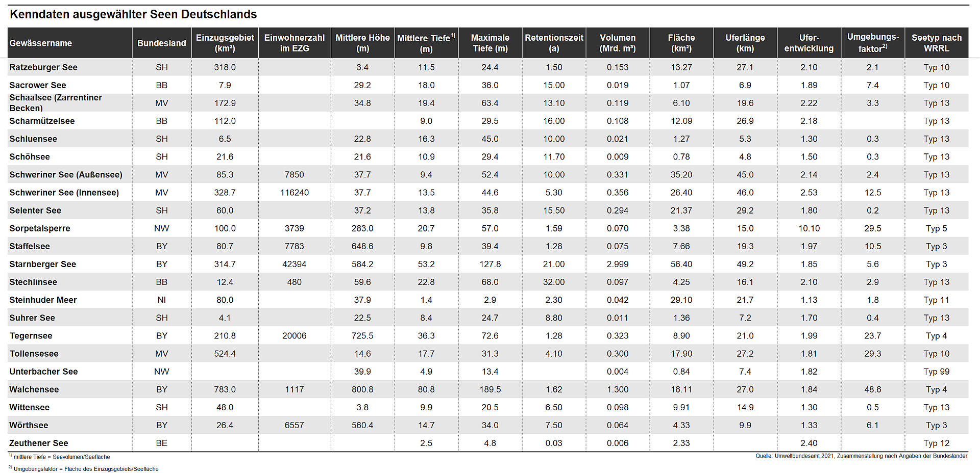
Example: A simplified subset from the UBA lake data

	name	shortname	z_mean	z_max	t_ret	volume	area	p_tot	n_no3	chl	wfd_type
Ammer	Ammersee	Ammer	37.60	81.1	2.70	1.75000	46.600	7.3	1.09	2.80	Typ 4
Arend	Arendsee	Arend	28.60	48.7	50.00	0.14700	5.140	375.0	0.05	22.30	Typ 13
Boden	Bodensee	Boden	85.00	254.0	4.20	48.52150	571.500	6.9	0.84	2.10	Typ 4
Chiem	Chiemsee	Chiem	25.60	73.4	1.26	2.04800	79.900	9.2	0.55	3.80	Typ 4
Dober	Dobersdorfer See	Dober	5.40	18.8	2.30	0.01690	3.120	63.9	0.64	27.30	Typ 14
Muegg	Großer Müggelsee	Muegg	4.85	7.5	0.20	0.03500	7.200	189.9	0.17	32.90	Typ 11
Ploen	Großer Plöner See	Ploen	12.40	58.0	3.10	0.37200	29.970	62.3	0.22	8.80	Typ 13
Kumme	Kummerower See	Kumme	8.10	23.3	1.50	0.26300	32.500	65.3	0.78	16.60	Typ 11
Mueritz	Müritz (Außenmüritz)	Mueritz	6.50	28.1	6.00	0.68000	105.300	19.7	0.11	6.30	Typ 14
MuerB	Müritz (Binnenmüritz)	MuerB	9.80	30.3	6.00	0.03800	3.910	34.2	0.11	6.70	Typ 10
Plaue	Plauer See	Plaue	6.80	25.5	3.00	0.30000	38.400	26.0	0.09	6.80	Typ 10
Sacro	Sacrower See	Sacro	18.01	36.0	15.00	0.01930	1.072	79.8	0.04	8.60	Typ 10
Schar	Scharmützelsee	Schar	9.00	29.5	16.00	0.10823	12.090	35.3	0.12	10.40	Typ 13
SchwA	Schweriner See (Außensee)	SchwA	9.40	52.4	10.00	0.33100	35.200	100.0	0.23	11.70	Typ 13
SchwI	Schweriner See (Innensee)	SchwI	13.50	44.6	5.30	0.35600	26.400	246.5	0.19	5.86	Typ 13
Starn	Starnberger See	Starn	53.20	127.8	21.00	2.99900	56.400	5.9	0.32	1.84	Typ 3
Stech	Stechlinsee	Stech	22.80	68.0	32.00	0.09700	4.250	15.8	0.04	2.60	Typ 13
Stein	Steinhuder Meer	Stein	1.35	2.9	2.30	0.04200	29.100	53.3	0.12	29.00	Typ 11

mean and maximum depth (\(\mathrm{m}\)): z_mean, z_max; retention time (years): t_ret; volume (\(\mathrm{10^9 m^3}\)); area (\(\mathrm{km^2}\)), total phosphorus P (\(\mathrm{\mu g/L}\)): p_tot; nitrogen-N (\(\mathrm{mg/L}\)): n_no3, chlorophyll (\(\mathrm{\mu g/L}\)): chl, water framework directive lake type: wfd_type

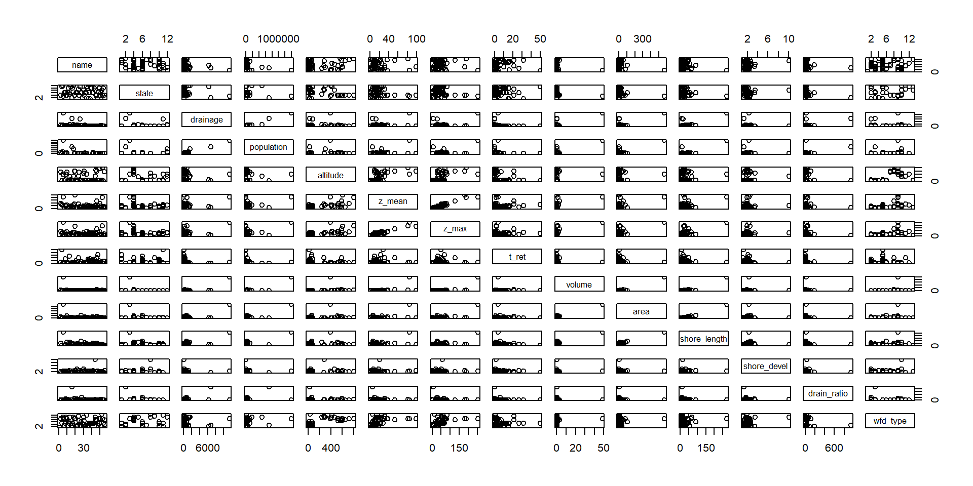
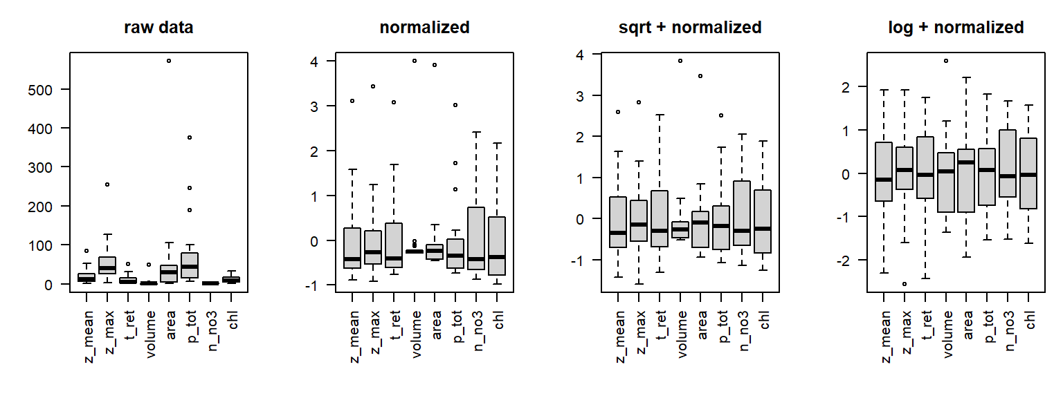
Data set from UBA (Umweltbundesamt = German Federal Environmental Agency), data modified
Original data source: https://www.umweltbundesamt.de/themen/wasser/seen
Terms of use: https://www.umweltbundesamt.de/datenschutz-haftung-urheberrecht

Code to read the data

lakes <- read.csv("https://tpetzoldt.github.io/datasets/data/lakes-combined-data.csv")
valid_columns <- c("name", "shortname", "z_mean", "z_max",  "t_ret", "volume", 
  "area", "p_tot", "n_no3", "chl", "wfd_type")
lakes <- lakes[valid_columns] |> na.omit()
row.names(lakes) <- lakes$shortname

lake_ids <- lakes[c("name", "shortname")]
lakedata <- lakes[, -c(1, 2)]

## remove wfd_type for now
lakedata$wfd_type <- NULL

• Source of original data: Uwweltbundesamt https://www.uba.de
• Data files downloadable from https://github.com/tpetzoldt/elements/tree/main/data/uba
• Terms of use, see: Copyright and description of derived data

Data transformation and normalization

par(mfrow = c(1, 4), mar = c(6, 4, 3, 1), las = 2)
boxplot(lakedata, main = "raw data")
boxplot(scale(lakedata), main = "normalized")
boxplot(scale(sqrt(lakedata)), main = "sqrt + normalized")
boxplot(scale(log(lakedata)), main = "log + normalized")

• scale() performs normalisation (z-transformation)
• aim: make different scales better comparable

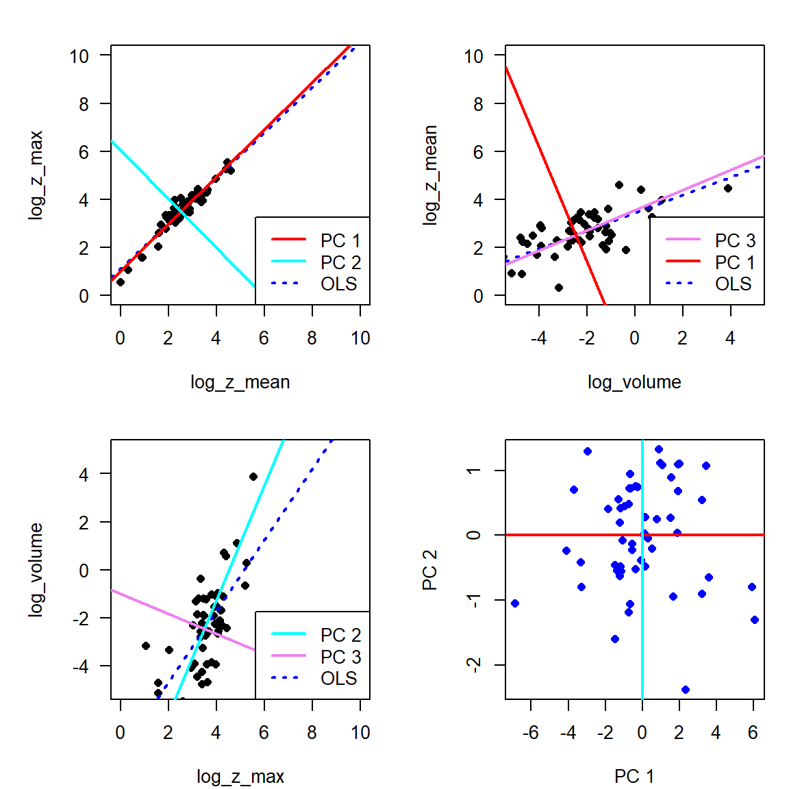
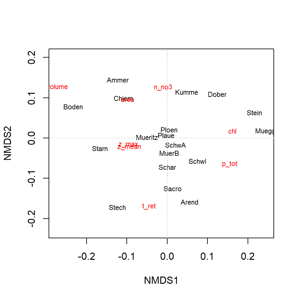
Ordination methods

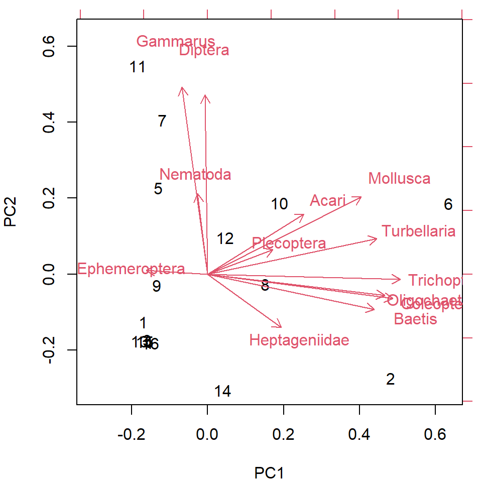
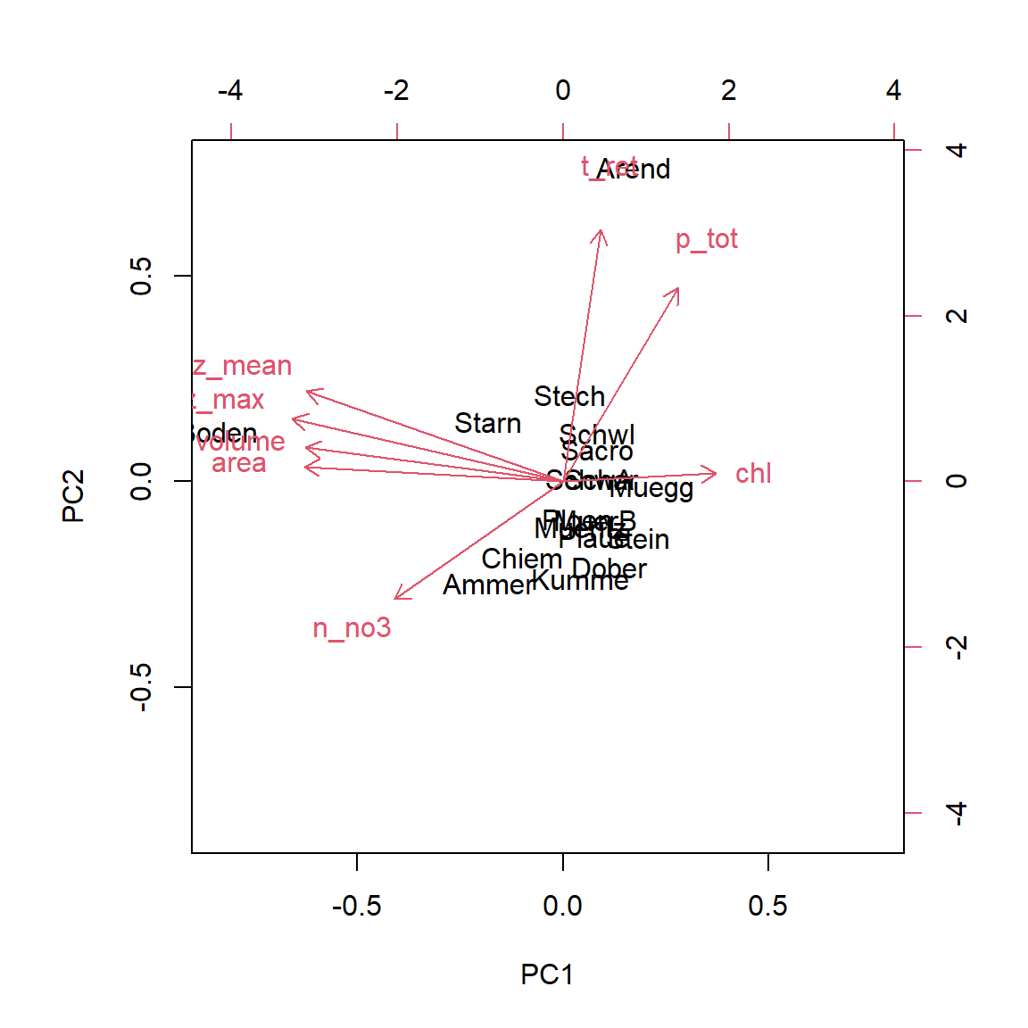
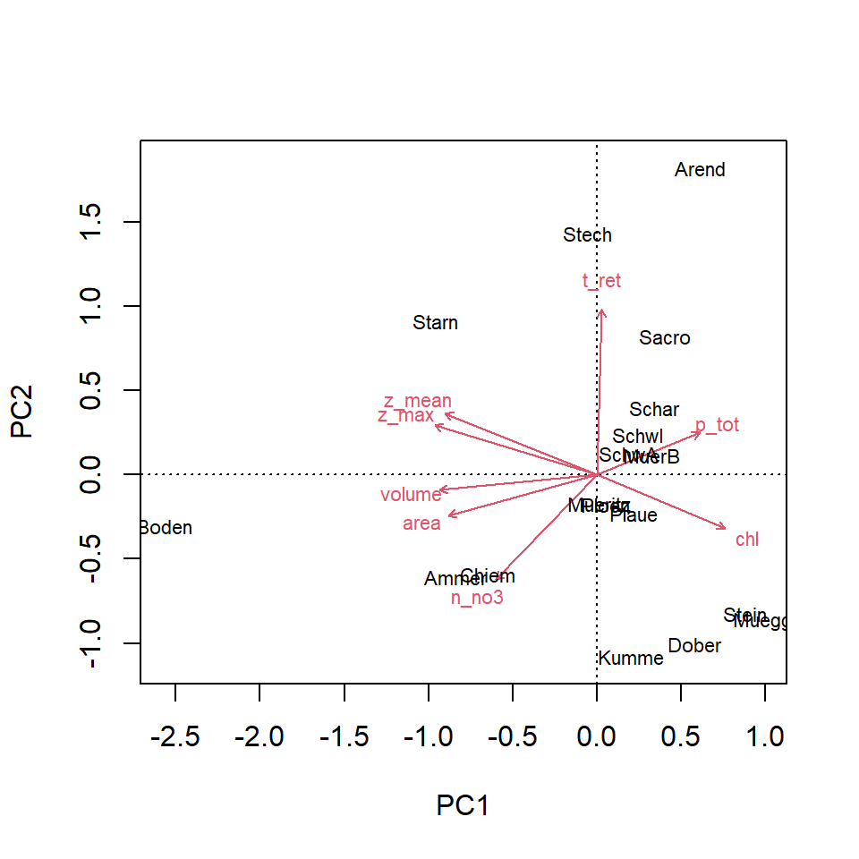
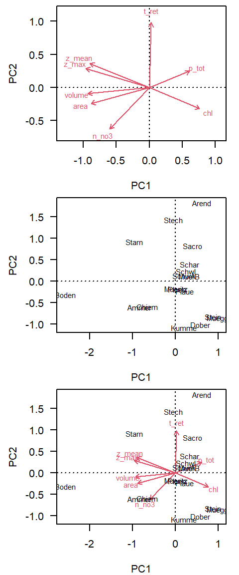
Principal Component Analysis: PCA

• identify cvovariance or correlation structure
• rotate coordinate system, so that it points in the diretions of maximum variance
• \(k\) dimensions in original space are transformed into \(k\) orthogonal (rectangular) coordinates in principal components space.
• works with any number of dimensions
• visualisation by a 3D example

Correlation structure of the lakes data set

round(cor(lakedata), 2)

       z_mean z_max t_ret volume  area p_tot n_no3   chl
z_mean   1.00  0.97  0.20   0.81  0.78 -0.17  0.48 -0.49
z_max    0.97  1.00  0.07   0.88  0.87 -0.26  0.47 -0.54
t_ret    0.20  0.07  1.00  -0.12 -0.18  0.48 -0.41 -0.04
volume   0.81  0.88 -0.12   1.00  0.98 -0.20  0.44 -0.27
area     0.78  0.87 -0.18   0.98  1.00 -0.26  0.45 -0.32
p_tot   -0.17 -0.26  0.48  -0.20 -0.26  1.00 -0.32  0.47
n_no3    0.48  0.47 -0.41   0.44  0.45 -0.32  1.00 -0.15
chl     -0.49 -0.54 -0.04  -0.27 -0.32  0.47 -0.15  1.00

• Let’s pick 3 variables for a 3D visualization: z_mix, z_max and volume.
• Use log-transformation to make them symetrically distributed.

z_mix, z_max and volume are highly corelated

\(\rightarrow\) We see that the three variables carry redundant information.

How rotation of axes works

Original coordinates

PCA rotated coordinates

• This slide contains interactive 3D graphics, that can be rotated with the mouse.
• Rotate the left image, so that the points on both size show similar patterns.
• Rotate the right image to show PC 3

\(\rightarrow\) Most of the 3D information of the data can be vizualized in 2D.

Note: log-transformed variables were used in this example.

PCA is an orthogonal (model II) regression

• PC1, PC2, PC3 are the principal components
• OLS is ordinary least squares regression (linear model lm)

Now analyse all numeric variables

	name	shortname	z_mean	z_max	t_ret	volume	area	p_tot	n_no3	chl
Ammer	Ammersee	Ammer	37.60	81.1	2.70	1.75000	46.600	7.3	1.09	2.80
Arend	Arendsee	Arend	28.60	48.7	50.00	0.14700	5.140	375.0	0.05	22.30
Boden	Bodensee	Boden	85.00	254.0	4.20	48.52150	571.500	6.9	0.84	2.10
Chiem	Chiemsee	Chiem	25.60	73.4	1.26	2.04800	79.900	9.2	0.55	3.80
Dober	Dobersdorfer See	Dober	5.40	18.8	2.30	0.01690	3.120	63.9	0.64	27.30
Muegg	Großer Müggelsee	Muegg	4.85	7.5	0.20	0.03500	7.200	189.9	0.17	32.90
Ploen	Großer Plöner See	Ploen	12.40	58.0	3.10	0.37200	29.970	62.3	0.22	8.80
Kumme	Kummerower See	Kumme	8.10	23.3	1.50	0.26300	32.500	65.3	0.78	16.60
Mueritz	Müritz (Außenmüritz)	Mueritz	6.50	28.1	6.00	0.68000	105.300	19.7	0.11	6.30
MuerB	Müritz (Binnenmüritz)	MuerB	9.80	30.3	6.00	0.03800	3.910	34.2	0.11	6.70
Plaue	Plauer See	Plaue	6.80	25.5	3.00	0.30000	38.400	26.0	0.09	6.80
Sacro	Sacrower See	Sacro	18.01	36.0	15.00	0.01930	1.072	79.8	0.04	8.60
Schar	Scharmützelsee	Schar	9.00	29.5	16.00	0.10823	12.090	35.3	0.12	10.40
SchwA	Schweriner See (Außensee)	SchwA	9.40	52.4	10.00	0.33100	35.200	100.0	0.23	11.70
SchwI	Schweriner See (Innensee)	SchwI	13.50	44.6	5.30	0.35600	26.400	246.5	0.19	5.86
Starn	Starnberger See	Starn	53.20	127.8	21.00	2.99900	56.400	5.9	0.32	1.84
Stech	Stechlinsee	Stech	22.80	68.0	32.00	0.09700	4.250	15.8	0.04	2.60
Stein	Steinhuder Meer	Stein	1.35	2.9	2.30	0.04200	29.100	53.3	0.12	29.00

• columns: called variables or species
• rows: observations or objects

PCA with the UBA lake data

pc <- prcomp(scale(lakedata))

Eigenvalues (proportion of variance) indicate importance of components.

summary(pc)

Importance of components:
                          PC1    PC2   PC3     PC4    PC5     PC6     PC7     PC8
Standard deviation     2.0692 1.2735 1.047 0.76067 0.5499 0.30497 0.12230 0.10618
Proportion of Variance 0.5352 0.2027 0.137 0.07233 0.0378 0.01163 0.00187 0.00141
Cumulative Proportion  0.5352 0.7379 0.875 0.94729 0.9851 0.99672 0.99859 1.00000

PCA Biplot

biplot(pc)

PCA with sqrt transformed data

lakedata2 <- sqrt(lakedata)
pc <- prcomp(scale(lakedata2))
summary(pc)

Importance of components:
                         PC1    PC2    PC3     PC4     PC5     PC6     PC7    PC8
Standard deviation     2.111 1.3059 0.9748 0.70830 0.50321 0.29742 0.17060 0.1266
Proportion of Variance 0.557 0.2132 0.1188 0.06271 0.03165 0.01106 0.00364 0.0020
Cumulative Proportion  0.557 0.7702 0.8889 0.95165 0.98330 0.99436 0.99800 1.0000

• The PCA with the untransformed data looked very asymmetric, we repeat it with square root transformed data.
• helps to get a better “resolution”
• must be taken into account when interpreting the results
• log transformation is also possible

Biplot of sqrt transformed data (1.-3. PC)

par(mfrow=c(1, 2), mar=c(5, 4, 4, 2.4), las=1)
biplot(pc)
biplot(pc, choices=c(3, 2))

PCA with the vegan package

pc <- rda(lakedata2, scale = TRUE)
summary(pc)

Call:
rda(X = lakedata2, scale = TRUE) 

Partitioning of correlations:
              Inertia Proportion
Total               8          1
Unconstrained       8          1

Eigenvalues, and their contribution to the correlations 

Importance of components:
                        PC1    PC2    PC3     PC4     PC5     PC6      PC7      PC8
Eigenvalue            4.456 1.7053 0.9503 0.50170 0.25322 0.08846 0.029105 0.016020
Proportion Explained  0.557 0.2132 0.1188 0.06271 0.03165 0.01106 0.003638 0.002003
Cumulative Proportion 0.557 0.7702 0.8889 0.95165 0.98330 0.99436 0.997997 1.000000

The two first PCs explain PC 1 = 77% of variance of the square root transformed observations.

Variance importance and biplot

Importance of components

• PC 1 = 56%
• PC 2 = 21%
• PC 3 = 12%

\(\Rightarrow\) The two first PCs explain PC 1 = 77% of variance of the square root transformed observations.

biplot(pc)

Interpretation

Variables

• only long arrows can be interpreted
• same direction: positive correlation
• opposite direction: negative correlation
• rectangular: no correlation

Observations

• identification of groups and extreme cases

Combined View

• relative size of variable for observations
• arrow direction: high values
• opposite direction: low values
• around middle: average

\(\Rightarrow\) Important: always read perpendicular to PCs and arrows!

Biplot in 3D

Variance

• PC 1 = 56%
• PC 2 = 21%
• PC 3 = 12%
• sum of PC 4 … 8 = 11%

\(\rightarrow\) Use the mouse to rotate and zoom.

Nonmetric Multidimensional Scaling: NMDS

md <- metaMDS(lakedata2, scale = TRUE, distance = "euclid", trace=FALSE)
plot(md, type="text")
abline(h=0, col="grey", lty="dotted")
abline(v=0, col="grey", lty="dotted")

The NMDS tries to map the higher dimensions even better to 2D or 3D. However, it accepts some distortion. More about this in the next chapter.

The code

lakes <- read.csv("https://tpetzoldt.github.io/datasets/data/lakes-combined-data.csv")
valid_columns <- c("name", "shortname", "z_mean", "z_max",  "t_ret", "volume", 
  "area", "p_tot", "n_no3", "chl", "wfd_type")

# set row names and limit data set to complete records without missing data
row.names(lakes) <- lakes$shortname
lakes <- na.omit(lakes[valid_columns])

# only the numerical variables
lakedata <- lakes[c("z_mean", "z_max",  "t_ret", "volume", 
                     "area", "p_tot", "n_no3", "chl")] 

## PCA with the vegan package
library("vegan")
lakedata2 <- sqrt(lakedata)
pc <- rda(lakedata2, scale = TRUE)
summary(pc)
biplot(pc)
biplot(pc, choices=c(3, 2))

## 3D Plot
library("vegan3d")
ordirgl(pc, col = "yellow")
orgltext(pc, display = "species", col="red")
orgltext(pc, display = "sites", col="blue", pos=4)
view3d(theta = 5, phi = 15, fov=30, zoom=1)

## NMDS
md <- metaMDS(lakedata2, scale = TRUE, distance = "euclid", trace=FALSE)
plot(md, type="text")
abline(h=0, col="grey", lty="dotted")
abline(v=0, col="grey", lty="dotted")

• Data and full source code is available from https://github.com/tpetzoldt/elements/

Summary

• Multivariate methods can be used to analyze data sets, where multiple variables depend on each other.
• PCA is a dimension reduction technique that tries to map high-dimensional data to a lower number of dimensions.
• It can be used as an explorative technique to find relationships between data.
• Compared to creating multiple plots between all variables, it helps to see the overall picture, saves time and avoids statistical fishing.
• The next chapter will introduce more methods.

Further reading

• Oksanen (2010)
• Borcard et al. (2018)

References

Borcard, D., Gillet, F., & Legendre, P. (2018). Numerical ecology with R. Springer International Publishing. https://doi.org/10.1007/978-3-319-71404-2

Oksanen, J. (2010). Multivariate analysis of ecological communities in R: Vegan tutorial.

Umweltbundesamt. (2021). Kenndaten ausgewählter Seen Deutschlands. https://www.umweltbundesamt.de/daten/wasser/zustand-der-seen#okologischer-zustand-der-seen

Winkelmann, C., Hellmann, C., Worischka, S., Petzoldt, T., & Benndorf, J. (2011). Fish predation affects the structure of a benthic community. Freshwater Biology, 56(6), 1030–1046. https://doi.org/10.1111/j.1365-2427.2010.02543.x