library(Kendall)
data(PrecipGL)
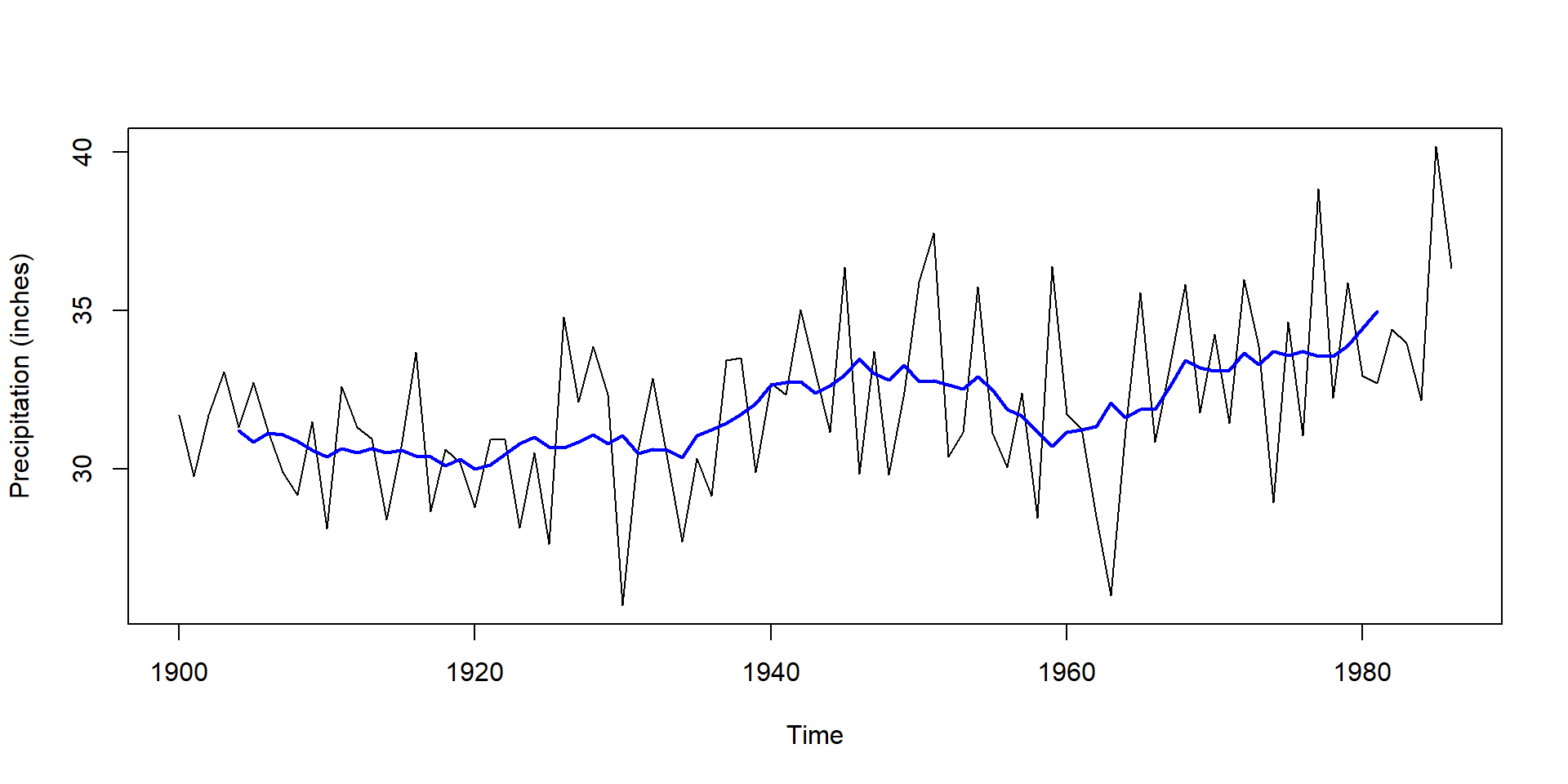
plot(PrecipGL, ylab="Precipitation (inches)")
# moving average with rectangular kernel
kernel <- rep(1, 10) # change second value to play with bandwidth
lines(stats::filter(PrecipGL, kernel/sum(kernel)), lwd = 2, col = "blue")10-Time Series Outlook
Applied Statistics – A Practical Course
2026-01-28
Smoothing methods
- alternative to parametric linear or non-linear regression vs. time
- smoothers are based on moving averages
Example: Annual precipitation 1900-1986, Great Lakes
Trend corrected series
smooth <- stats::filter(PrecipGL, kernel/sum(kernel))
residuals <- PrecipGL - smooth
plot(residuals)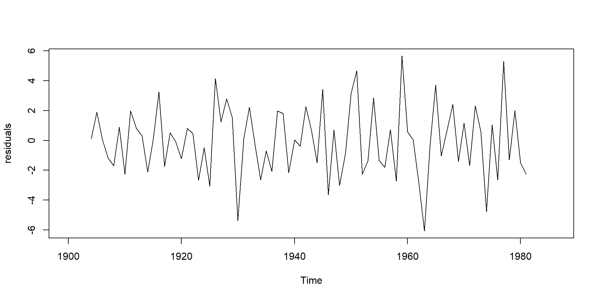
- Trend corrected series can be obtained by subtracting the trend.
- Note: use
stats::filterto avoid potential conflict withdplyr::filter.
Smoothing of data with 12monthly seasonality
- For a seasonal time series with monthly values Kleiber & Zeileis (2008) recommend a filter with 13 coefficients.
- Example: water level of Rio Negro 18 km upstream from its confluence with the Amazon River.
- The data set is contained in the package boot (Canty & Ripley, 2022):
library(boot)
data(manaus)
tsp(manaus) # shows time series properties
[1] 1903.000 1992.917 12.000plot(manaus)
lines(stats::filter(manaus, c(0.5, rep(1, 11), 0.5)/12), lwd=2, col="blue")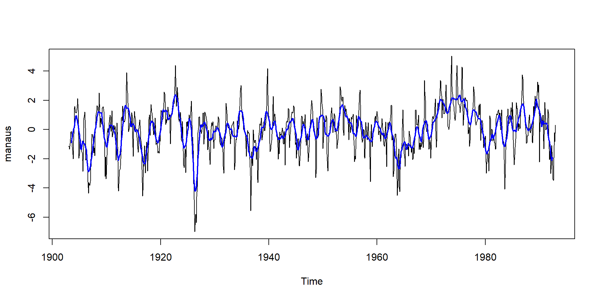
Very popular method: The LOWESS filter
Show the code
plot(PrecipGL)
lines(lowess(time(PrecipGL), PrecipGL, f = 2/3), lwd = 3, col = "blue")
lines(lowess(time(PrecipGL), PrecipGL, f = 1/3), lwd = 3, col = "forestgreen")
lines(lowess(time(PrecipGL), PrecipGL, f = 0.1), lwd = 3, col = "red")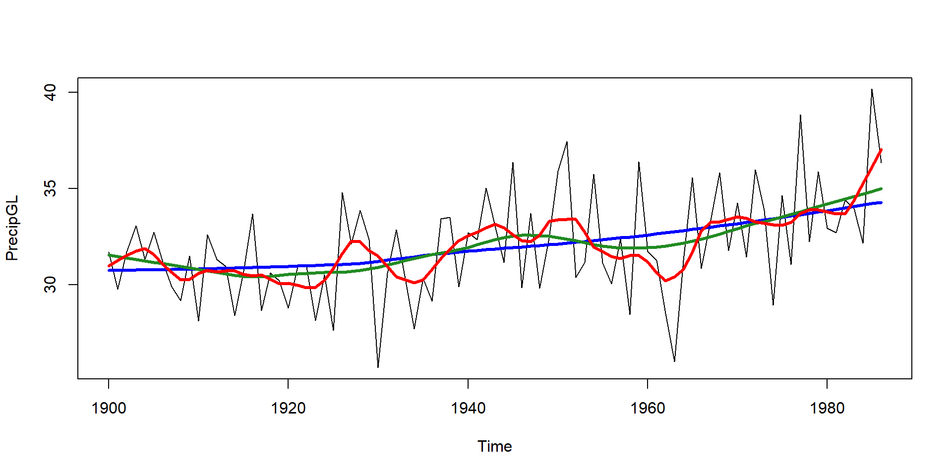
- locally weighted polynomial regression (W. S. Cleveland, 1979)
- allows to adjust smoothness (smoother span
f) - different functions available in R:
lowessandloess
Fast Fourier transform
Show the code
# create an arbitrary time series
set.seed(123)
n   <- 360
t   <- 0:(n-1)
x   <- sin(t*2*pi/n) + rnorm(n, sd = 0.2)
plot(t, x, xlim = c(-10, 370))

# perform the FFT
p       <- fft(x)

# invert the FFT for the main period only (keep parameters 1..3)
p[4:n]  <- 0 # set higher order parameters to zero
x_sim      <- fft(p, inverse = TRUE)
lines(t, 2 * Re(x_sim)/n - Re(p[1])/n, col = "blue", lwd = 4)


## perform FFT and invert it for all periods
p       <- fft(x)
p[(n/2):n] <- 0 # set only the "redundant frequencies" to zero
x_sim         <- fft(p, inverse = TRUE)
lines(t, 2 * Re(x_sim)/n - Re(p[1])/n, col = "red", lwd = 1)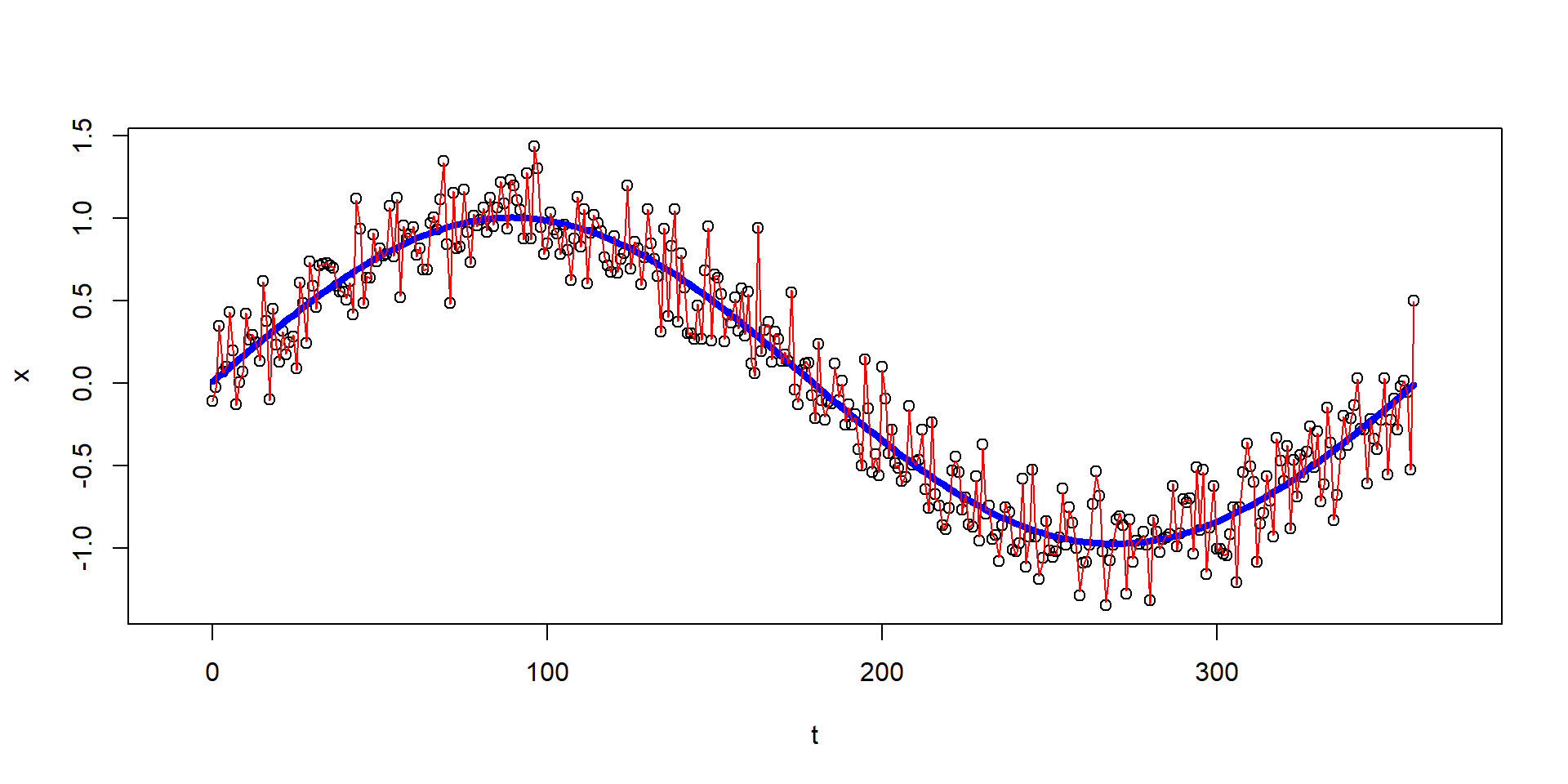
Automatic time series decomposition
Function decompose implements the classical approach with symmetric moving average.
manaus_dec <- decompose(manaus)
plot(manaus_dec)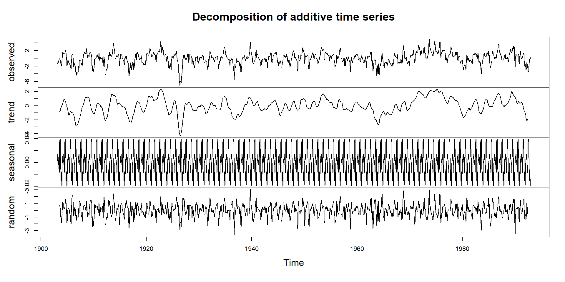
- In this data set the seasonal component possesses an additive character.
- In case of a multiplicative components, use
type = "multiplicative".
Automatic time series decomposition II
- function
stl(seasonal time series decomposition) (R. B. Cleveland et al., 1990) - uses a LOESS filter
manaus_stl <- stl(manaus, s.window=13)
plot(manaus_stl)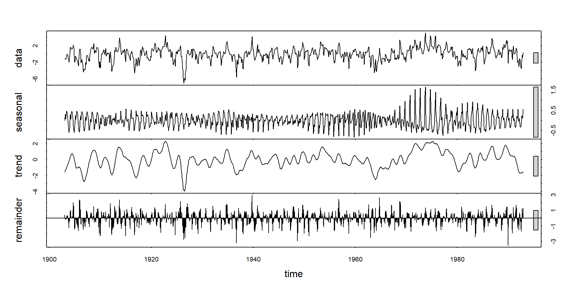
Example: SARIMA model for CO2 in the atmosphere
Show the code
## read data directly from NOAA
#co2 <- read_csv("https://gml.noaa.gov/webdata/ccgg/trends/co2/co2_mm_mlo.csv",
#                skip = 40, show_col_types = FALSE)

## local version
co2 <- read_csv("../data/co2_mm_mlo.csv", skip=40, show_col_types = FALSE)

## year 1958 is incomplete, so let's start with 1959
co2 <- dplyr::filter(co2, year > 1958)

co2 |>
  mutate(date=as_date(paste(year, month, 15, sep="."))) |>
  ggplot(aes(date, average)) +
  geom_line() + ylab(expression(CO[2]~"in the atmosphere (ppm)")) +
  ggtitle("Mauna Loa Observatory, Hawaii, Monthly Averages") +
  geom_smooth()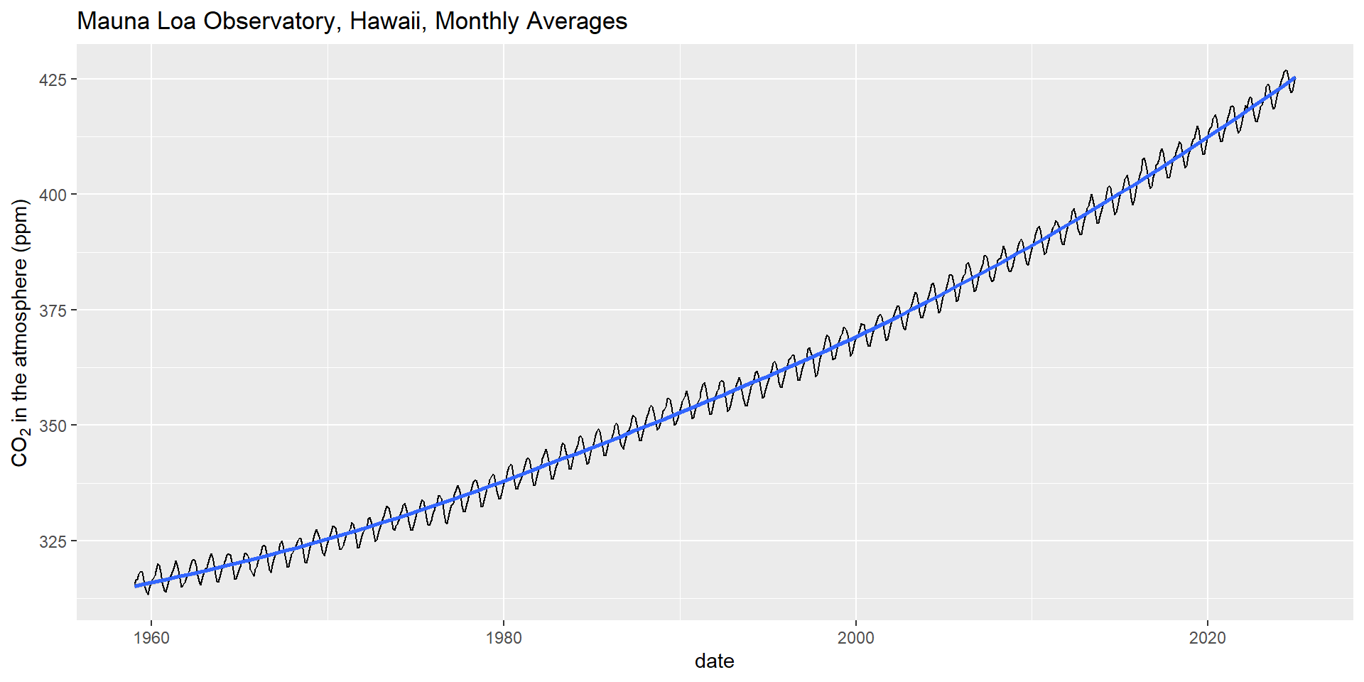
Fit SARIMA model to CO2 data
Show the code
library(astsa)

## convert to a time series object
co2ts <- ts(co2$average, start=1959, frequency = 12)

## fit a SARIMA model and show the results
m <- sarima(co2ts, p = 1, d = 1, q = 1, P = 0, D = 1, Q = 1, S = 12)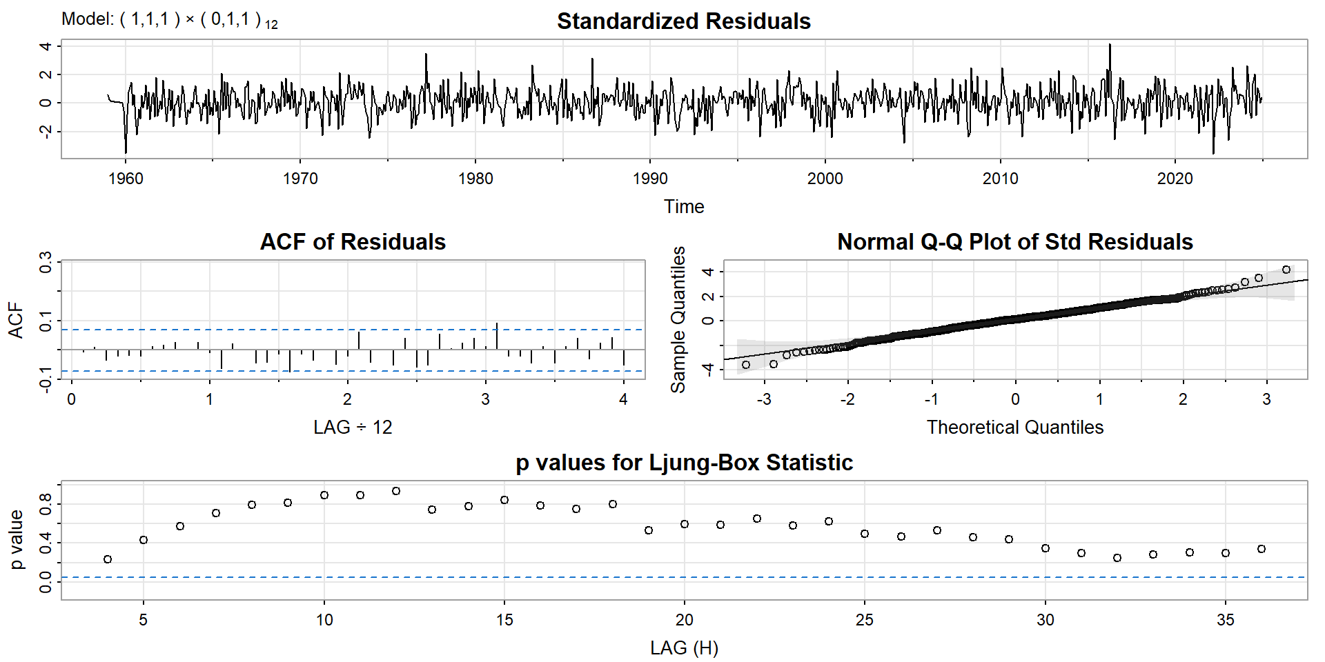
Mathematical details can be found in Shumway & Stoffer (2019).
SARIMA-forecast of CO2
Show the code
m <- sarima.for(co2ts, n.ahead = 12 * 27,
           p = 1, d = 1, q = 1, P = 0, D = 1, Q = 1, S = 12,
           plot.all = TRUE)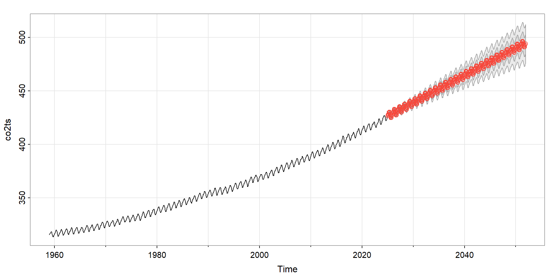
Mathematical details can be found in Shumway & Stoffer (2019).
Identification of structural breaks
Structural break
If one or more statistical parameters are not constant over the whole length of a time series it is called a structural break. For instance a location parameter (e.g. the mean), a trend or another distribution parameter (such as variance or covariance) may change.
Testing for structural breaks
The package strucchange implements a number of tests for identification of structural changes or parameter instability of time series. Generally, two approaches are available: fluctuation tests and F-based tests. Fluctuation tests try to detect the structural instability with cumulative or moving sums (CUSUMs and MOSUMs).
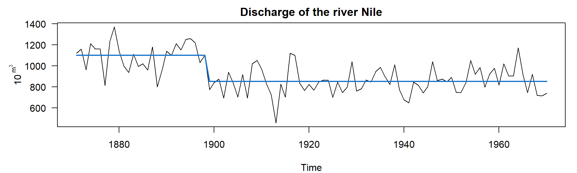
The Nile data set
The Nile data set contains measurements of annual discharge of the Nile at Aswan from 1871 to 1970 (see help page ?Nile for data source):
library(strucchange)
data("Nile")
plot(Nile)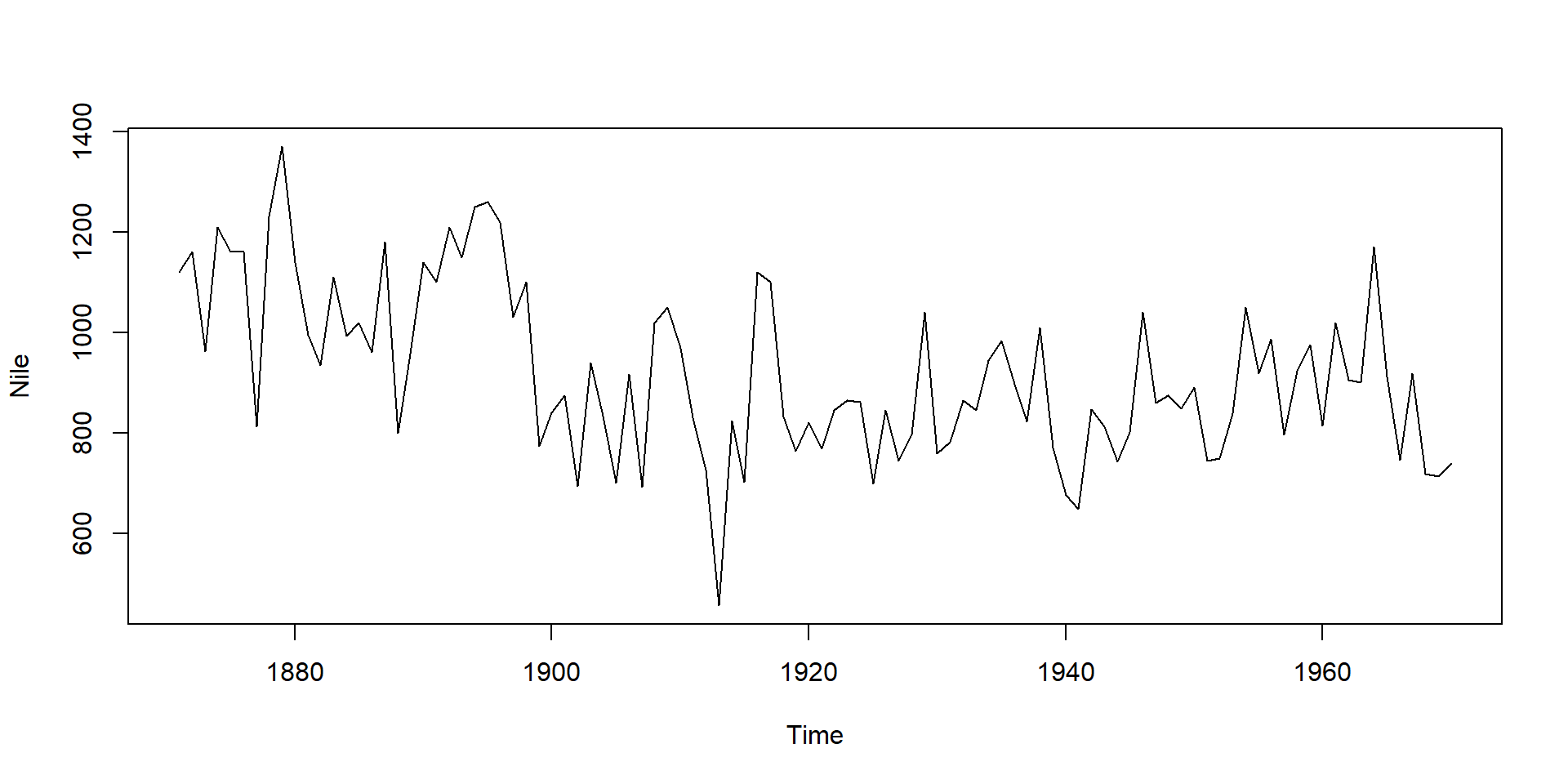
Test for existence of structural break
- Are there are periods with different flow?
- use of OLS-CUSUM (ordinary least squares, cumulative sum) or MOSUM tests (moving average sum)
efp= empirical fluctuation process,sctest= structural change test
ocus <- efp(Nile ~ 1, type = "OLS-CUSUM")
plot(ocus)sctest(ocus)
    OLS-based CUSUM test

data:  ocus
S0 = 2.9518, p-value = 5.409e-08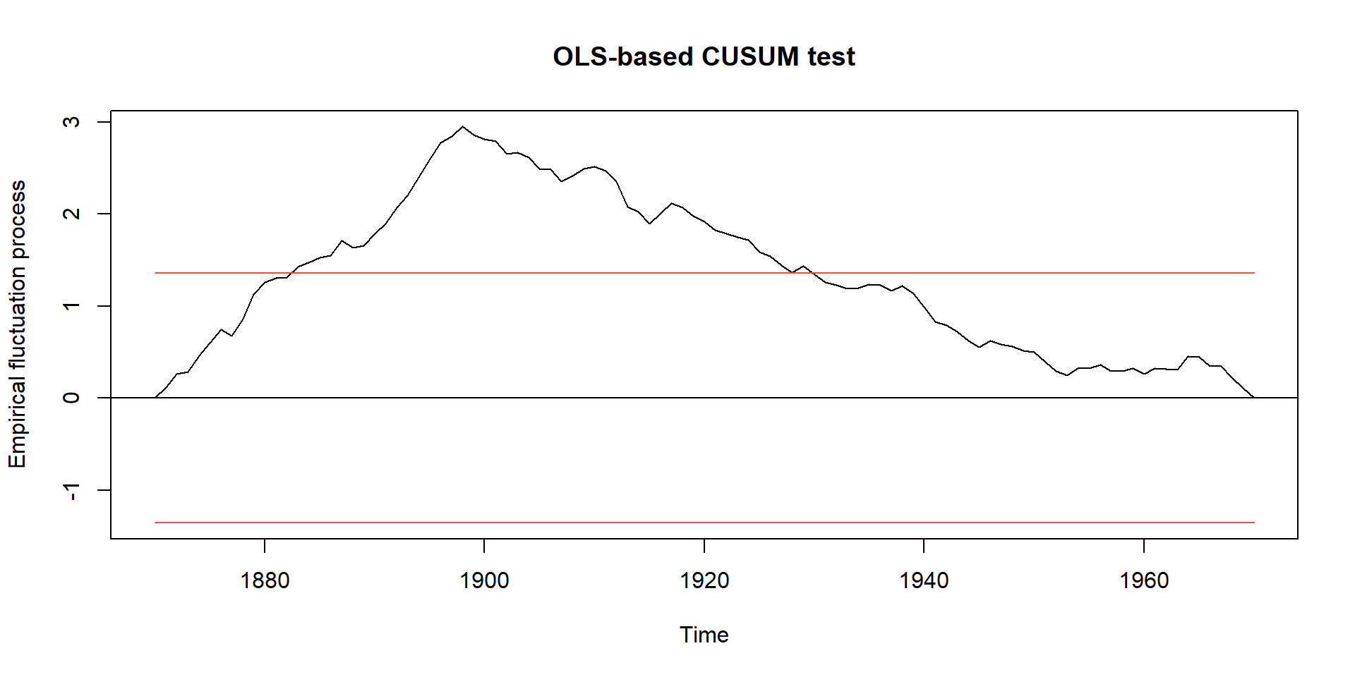
Likelihood profile: \(\rightarrow\) optimal number of breaks?
bp.nile <- breakpoints(Nile ~ 1)
plot(bp.nile)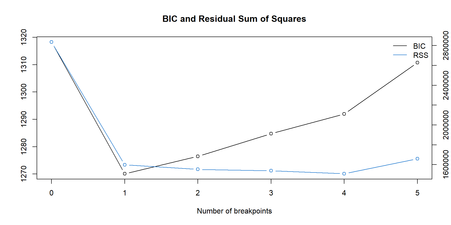
- RSS (residual sum of squares) shows goodness of fit. The smaller the better.
- Penalty = 2 \(\cdot\) number of breakpoints (not shown).
- Minimum BIC indicates optimal model.
Plot breakpoints and confidence interval
## fit null hypothesis model and model with 1 breakpoint
fm0 <- lm(Nile ~ 1)
fm1 <- lm(Nile ~ breakfactor(bp.nile,  breaks = 1))
plot(Nile)
lines(ts(fitted(fm0),  start = 1871),  col = 3)
lines(ts(fitted(fm1),  start = 1871),  col = 4)
lines(bp.nile)

## confidence interval
ci.nile <- confint(bp.nile)
#ci.nile  # output numerical results
lines(ci.nile)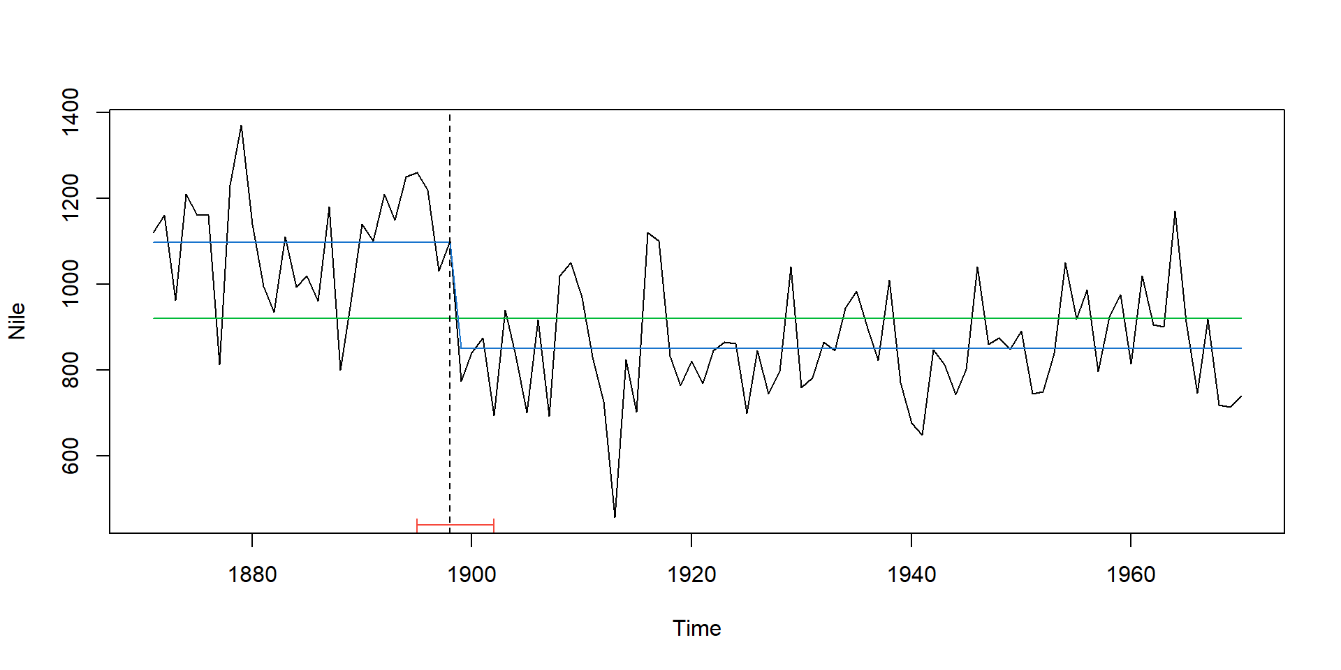
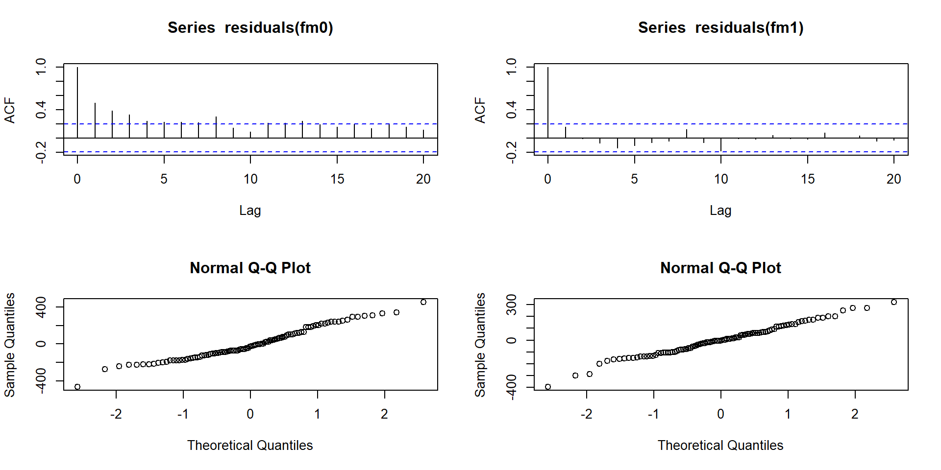
Diagnostics
par(mfrow = c(2, 2))
acf(residuals(fm0))     # model without breaks
acf(residuals(fm1))     # model with 1 breakpoint
qqnorm(residuals(fm0))
qqnorm(residuals(fm1))