07-One and two-way ANOVA

Applied Statistics – A Practical Course

Thomas Petzoldt

2025-02-08

ANOVA – Analysis of Variances

• Testing of complex hypothesis as a whole, e.g.:
  • more than two samples (multiple test problem),
  • several multiple factors (multiway ANOVA)
  • elimination of covariates (ANCOVA)
  • fixed and/or random effects (variance decomposition methods, mixed effects models)
• Different application scenarios:
  • explorative use: Which influence factors are important?
  • descriptive use: Fitting of models for process description and forecasting.
  • significance tests.
• ANOVA methods are (in most cases) based on linear models.

A practical example

Find a suitable medium for growth experiments with green algae

• cheap, easy to handle
• suitable for students courses and classroom experiments

Idea

• use a commercial fertilizer with the main nutrients N and P
• mineral water with trace elements
• does non-sparkling mineral water contain enough \(\mathrm{CO_2}\)?
• test how to improve \(\mathrm{CO_2}\) availability for photosynthesis

Application

7 Different treatments

1. fertilizer solution in closed bottles
2. fertilizer solution in open bottles (\(\mathrm{CO_2}\) from air)
3. fertilizer + sugar (organic C source)
4. fertilizer + additional \(\mathrm{HCO_3^-}\) (add \(\mathrm{CaCO_3}\) to sparkling mineral water)
5. a standard algae growth medium (“Basal medium”) for comparison
6. deionized (“destilled”) water and
7. tap water for comparison

Experimental design

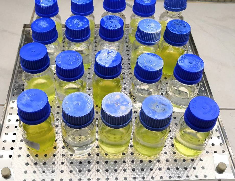
• each treatment with 3 replicates
• randomized placement on a shaker
• 16:8 light:dark-cycle
• measurement directly in the bottles using a self-made turbidity meter

Results

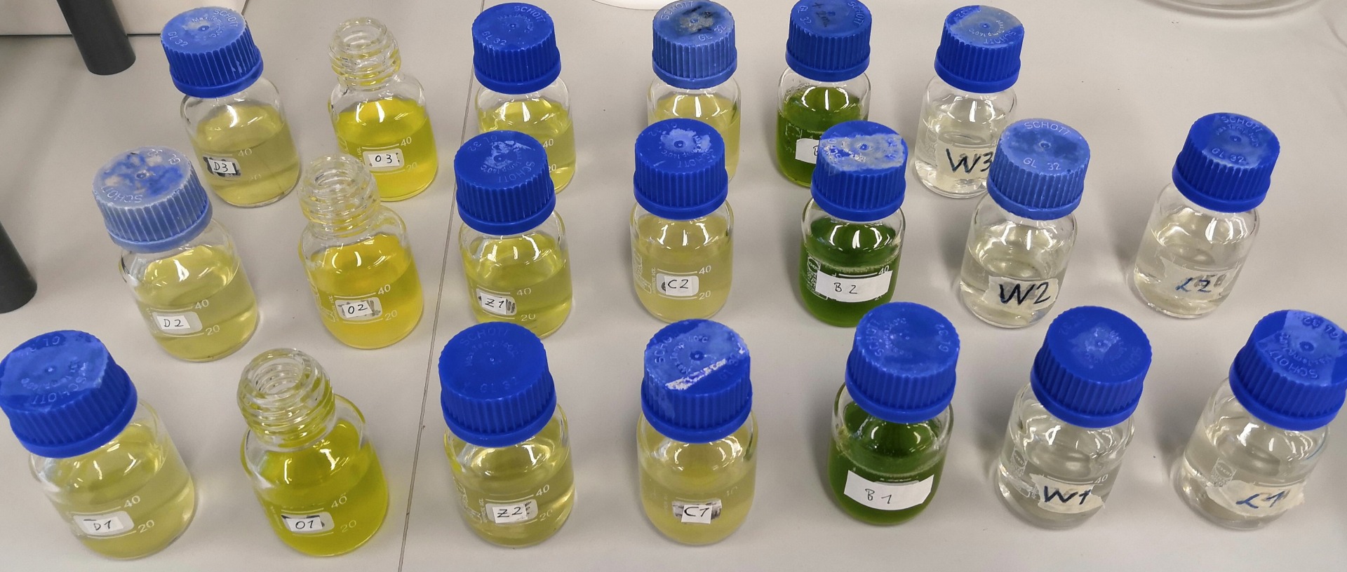Fertilizer – Open Bottle – F. + Sugar – F. + CaCO3 – Basal medium – A. dest – Tap water

The data set

Table 1: Growth from day 2 to day 6 (relative units)

treat	replicate 1	replicate 2	replicate 3
Fertilizer	0.020	-0.217	-0.273
F. open	0.940	0.780	0.555
F.+sugar	0.188	-0.100	0.020
F.+CaCO3	0.245	0.236	0.456
Bas.med.	0.699	0.727	0.656
A.dest	-0.010	0.000	-0.010
Tap water	0.030	-0.070	NA

• NA means “not available”, i.e. a missing value
• the crosstable structure is compact and easy to read, but not ideal for data analysis
• \(\Rightarrow\) convert it to long format

Data in long format

Advantages

• looks “stupid” but is better for data analysis
• dependent variable growth and
  explanation variable treat clearly visible
• model formula: growth ~ treat
• easily extensible to \(>1\) explanation variable

treat	rep	growth
Fertilizer	1	0.020
Fertilizer	2	-0.217
Fertilizer	3	-0.273
F. open	1	0.940
F. open	2	0.780
F. open	3	0.555
F.+sugar	1	0.188
F.+sugar	2	-0.100
F.+sugar	3	0.020
F.+CaCO3	1	0.245
F.+CaCO3	2	0.236
F.+CaCO3	3	0.456

The data in R

algae <- data.frame(
  treat  = factor(c("Fertilizer", "Fertilizer", "Fertilizer", 
             "F. open", "F. open", "F. open", 
             "F.+sugar", "F.+sugar", "F.+sugar", 
             "F.+CaCO3", "F.+CaCO3", "F.+CaCO3", 
             "Bas.med.", "Bas.med.", "Bas.med.", 
             "A.dest", "A.dest", "A.dest", 
             "Tap water", "Tap water"),
             levels=c("Fertilizer", "F. open", "F.+sugar", 
                    "F.+CaCO3", "Bas.med.", "A.dest", "Tap water")),
  rep   = c(1, 2, 3, 1, 2, 3, 1, 2, 3, 1, 2, 3, 1, 2, 3, 1, 2, 3, 1, 2), 
  growth = c(0.02, -0.217, -0.273, 0.94, 0.78, 0.555, 0.188, -0.1, 0.02, 
             0.245, 0.236, 0.456, 0.699, 0.727, 0.656, -0.01, 0, -0.01, 0.03, -0.07)
)

… can be entered directly in the code. A csv-file in long format is also possible.

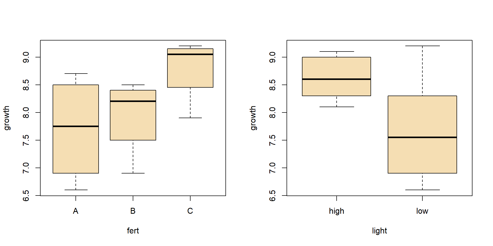
Boxplot

boxplot(growth ~ treat, data = algae)
abline(h = 0, lty = "dashed", col = "grey")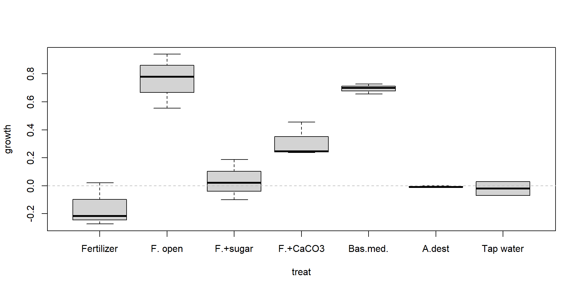

Stripchart

stripchart(growth ~ treat, data = algae, vertical = TRUE)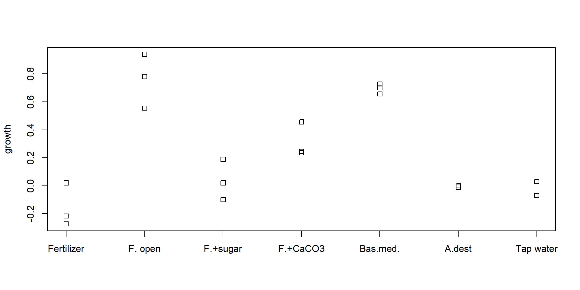

Better, because we have only 2-3 replicates. Boxplot needs more.

Turn scientific question into a statistical hypothesis

Scientific Questions

• Are the treatments different?
• Which medium is the best?
• Is the best medium significantly better than the others?

Statistical Hypotheses

• \(H_0\): growth is the same in all treatments
• \(H_A\): differences between media

Why can’t we apply just several t-tests?

• If we have 7 treatments and want to test all against each other, we would need:

\[7 \cdot (7 - 1) / 2 = 21 \qquad\text{tests.}\]

• If we set \(\alpha = 0.05\) we get 5% false positives. \(\Rightarrow\) One of 20 tests is on average a false positive
• If we do \(N\) tests, we increase the overall \(\alpha\) error to \(N\cdot\alpha\) in the worst case.
• This is called alpha-error-inflation or the Bonferroni law:

\[ \alpha_{total} \le \sum_{i=1}^{N} \alpha_i = N \cdot \alpha \]

If we ignore the Bonferroni law, we end in statistical fishing and get spurious results just by chance.

Solutions

1. Down-correct the alpha errors so that \(\alpha_{total} = 0.05\).
   \(\rightarrow\) Bonferroni rule.
2. Use a method that does all tests simultanaeously: the ANOVA.

ANOVA: Analysis of variances

Basic Idea

• Split the total variance into effect(s) and errors:

\[ s_y^2 = s^2_\mathrm{effect} + s^2_{\varepsilon} \]

• Somewhat surprising: we use variances to compare mean values.
• Explanation: differences of means contribute to the total variance of the whole sample.
• Variance components can be called variance within (\(s^2_\varepsilon\)) and variance between samples.
• The way how to separate variances is a linear model.

Example

Two brands of Clementine fruits from a shop “E”, that we encode as “EB” and “EP”. We want to know whether the premium brand (“P”) and the basic brand (“B”) have a different weight.

clem <- data.frame(
  brand = c("EP", "EB", "EB", "EB", "EB", "EB", "EB", "EB", "EB", "EB", "EB", 
            "EB", "EB", "EB", "EP", "EP", "EP", "EP", "EP", "EP", "EP", "EB", "EP"),
  weight = c(88, 96, 100, 96, 90, 100, 92, 92, 102, 99, 86, 89, 99, 89, 75, 80, 
             81, 96, 82, 98, 80, 107, 88))

We encode one sample (“EB”) with 1 and the other sample (“EP”) with 2:

clem$code <- as.numeric(factor(clem$brand))
clem$code

 [1] 2 1 1 1 1 1 1 1 1 1 1 1 1 1 2 2 2 2 2 2 2 1 2

Then we fit a linear regression:

plot(weight ~ code, data = clem, axes = FALSE)
m <- lm(weight ~ code, data = clem)
axis(1, at = c(1,2), labels = c("EB", "EP")); axis(2); box()
abline(m, col = "blue")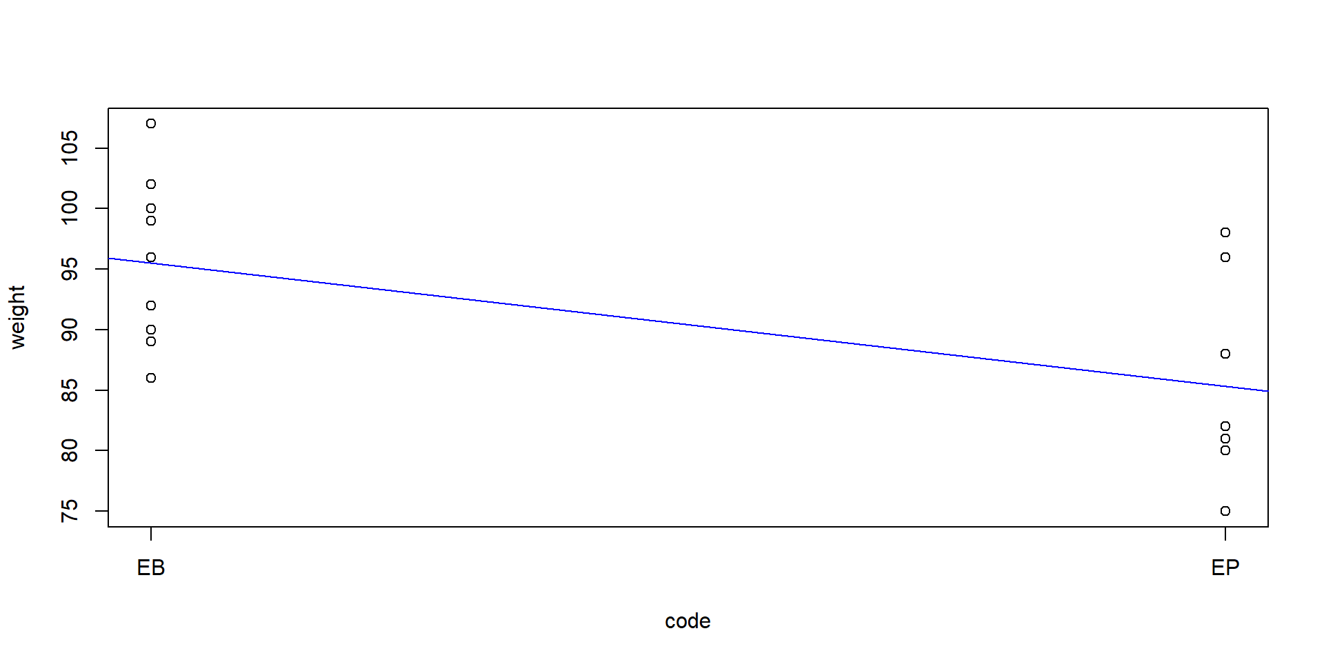

Variance components

We fit a linear model and compare the variances:

m <- lm(weight ~ code, data = clem)

total variance

(var_tot <- var(clem$weight))

[1] 68.98814

residual variance (= within variance)

(var_res <- var(residuals(m)))

[1] 43.25

explained variance (= between variance)

var_tot - var_res

[1] 25.73814

Now we can analyse whether the between variance is big enough to justify a significant effect.

This is called an ANOVA.

ANOVA

anova(m)

Analysis of Variance Table

Response: weight
          Df Sum Sq Mean Sq F value   Pr(>F)   
code       1 566.24  566.24  12.497 0.001963 **
Residuals 21 951.50   45.31                    
---
Signif. codes:  0 '***' 0.001 '**' 0.01 '*' 0.05 '.' 0.1 ' ' 1

A t-test for comparison

t.test(weight ~ code, data = clem, var.equal=TRUE)

    Two Sample t-test

data:  weight by code
t = 3.5351, df = 21, p-value = 0.001963
alternative hypothesis: true difference in means between group 1 and group 2 is not equal to 0
95 percent confidence interval:
  4.185911 16.147423
sample estimates:
mean in group 1 mean in group 2 
       95.50000        85.33333 

\(\Rightarrow\) the p-values are exactly the same.

ANOVA with more than 2 samples

Back to the algae growth data. Let’s call the linear model m:

m <- lm(growth ~ treat, data = algae)

• We can print the coefficients of the linear model with summary(m)
• But we are interested in the overall effect and use anova

anova(m)

Analysis of Variance Table

Response: growth
          Df  Sum Sq Mean Sq F value    Pr(>F)    
treat      6 2.35441 0.39240  25.045 1.987e-06 ***
Residuals 13 0.20368 0.01567                      
---
Signif. codes:  0 '***' 0.001 '**' 0.01 '*' 0.05 '.' 0.1 ' ' 1

• The ANOVA table shows F-tests testing for significance of all factors.
• In the table above, we have only one single factor.

\(\Rightarrow\) We see that the treatment had a significant effect.

Posthoc tests

• The test showed, that the factor “treatment” had a significant effect.
• We don’t know yet, which factor levels were different.

Tukey HSD test is the most common.

tk <- TukeyHSD(aov(m))
tk

  Tukey multiple comparisons of means
    95% family-wise confidence level

Fit: aov(formula = m)

$treat
                            diff         lwr         upr     p adj
F. open-Fertilizer    0.91500000  0.56202797  1.26797203 0.0000103
F.+sugar-Fertilizer   0.19266667 -0.16030537  0.54563870 0.5211198
F.+CaCO3-Fertilizer   0.46900000  0.11602797  0.82197203 0.0069447
Bas.med.-Fertilizer   0.85066667  0.49769463  1.20363870 0.0000231
A.dest-Fertilizer     0.15000000 -0.20297203  0.50297203 0.7579063
Tap water-Fertilizer  0.13666667 -0.25796806  0.53130140 0.8837597
F.+sugar-F. open     -0.72233333 -1.07530537 -0.36936130 0.0001312
F.+CaCO3-F. open     -0.44600000 -0.79897203 -0.09302797 0.0102557
Bas.med.-F. open     -0.06433333 -0.41730537  0.28863870 0.9943994
A.dest-F. open       -0.76500000 -1.11797203 -0.41202797 0.0000721
Tap water-F. open    -0.77833333 -1.17296806 -0.38369860 0.0001913
F.+CaCO3-F.+sugar     0.27633333 -0.07663870  0.62930537 0.1727182
Bas.med.-F.+sugar     0.65800000  0.30502797  1.01097203 0.0003363
A.dest-F.+sugar      -0.04266667 -0.39563870  0.31030537 0.9994197
Tap water-F.+sugar   -0.05600000 -0.45063473  0.33863473 0.9985686
Bas.med.-F.+CaCO3     0.38166667  0.02869463  0.73463870 0.0307459
A.dest-F.+CaCO3      -0.31900000 -0.67197203  0.03397203 0.0879106
Tap water-F.+CaCO3   -0.33233333 -0.72696806  0.06230140 0.1247914
A.dest-Bas.med.      -0.70066667 -1.05363870 -0.34769463 0.0001792
Tap water-Bas.med.   -0.71400000 -1.10863473 -0.31936527 0.0004507
Tap water-A.dest     -0.01333333 -0.40796806  0.38130140 0.9999997

Graphical output

par(las = 1)             # las = 1 make y annotation horizontal
par(mar = c(4, 10, 3, 1)) # more space at the left for axis annotation
plot(tk)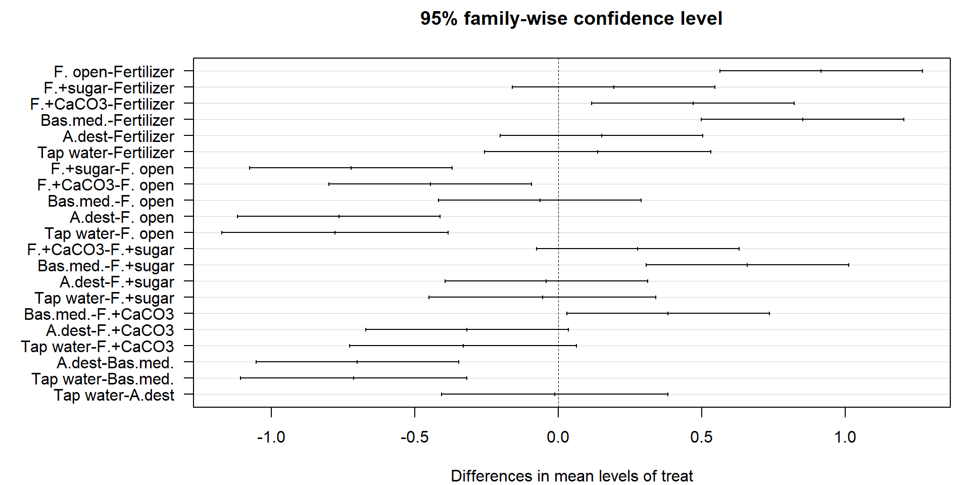

ANOVA assumptions and diagnostics

ANOVA has same assumptions as the linear model.

1. Independence of errors
2. Variance homogeneity
3. Approximate normality of errors

Graphical checks are preferred.

par(mfrow=c(2, 2))
plot(m)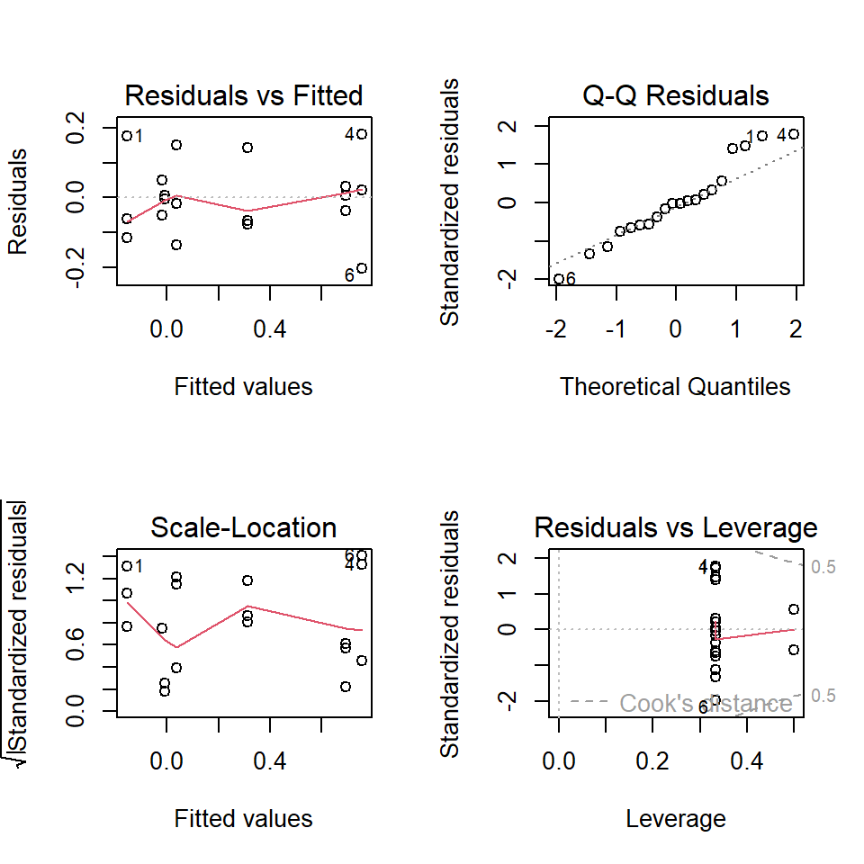

Numerical tests

Test variance homogeneity

• F-test compares only two variances.
• Several tests for multiple variances, e.g. Bartlett, Levene, Fligner-Killeen
• Recommended: Fligner-Killeen-test

fligner.test(growth ~ treat, 
             data = algae)

    Fligner-Killeen test of homogeneity of variances

data:  growth by treat
Fligner-Killeen:med chi-squared = 4.2095, df = 6, p-value = 0.6483

Test of normal distribution

• The Shapiro-Wilks test can be misleading.
• Use a graphical method!

qqnorm(residuals(m))
qqline(residuals(m))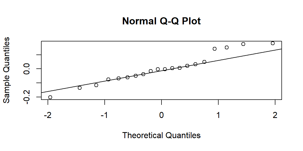

One-way ANOVA with heterogeneous variances

• extension of the Welch test for \(\ge 2\) samples
• in R called oneway.test

oneway.test(growth ~ treat, data = algae)

    One-way analysis of means (not assuming equal variances)

data:  growth and treat
F = 115.09, num df = 6.0000, denom df = 4.6224, p-value = 6.57e-05

Two-way ANOVA

• Example from a statistics text book (Crawley, 2002), applied to a new context
• Effects of fertilizer and light regime on growth of plant height in cm per time

fertilizer	high light	low light
A	8.3	6.6
A	8.7	7.2
B	8.1	6.9
B	8.5	8.3
C	9.1	7.9
C	9.0	9.2

• factorial experiment (with replicates): each factor combination has more than one observation.
• without replication:
  • no replicates per factor combination
  • this is possible, but does not allow identification of interactions

Enter data in long format

plants <- data.frame(No = 1:12,
                    growth = c(6.6, 7.2, 6.9, 8.3, 7.9, 9.2,
                               8.3, 8.7, 8.1, 8.5, 9.1, 9.0),
                    fert   = rep(c("A", "B", "C"), each=2),
                    light   = rep(c("low", "high"), each=6)
          )

No	growth	fert	light
1	6.6	A	low
2	7.2	A	low
3	6.9	B	low
4	8.3	B	low
5	7.9	C	low
6	9.2	C	low
7	8.3	A	high
8	8.7	A	high
9	8.1	B	high
10	8.5	B	high
11	9.1	C	high
12	9.0	C	high

Model formula examples

Model Type	Formula
Null model	y ~ 1
Simple linear regression	y ~ x
Linear model without intercept	y ~ x - 1
Multiple regression, no interaction	y ~ x1 + x2 + x3
Multiple regression with interaction	y ~ x1 * x2 * x3
Multiple regression, no 3x interaction	y ~ x1 * x2 * x3 - x1 : x2 : x3
Transformed with ‘as is’ function	y ~ x + I(x^2)
One way ANOVA	y ~ f
ANOVA with interaction	y ~ f1 * f2
ANCOVA with Interaction	y ~ x * f
Nested ANOVA	y ~ x + (1 | a / b)
GAM with smoother s	y ~ s(x) + f

• y = response variable (dependent, target)
• x = metric explanation variable (predictor, independent); f = factor variable (nominal)

Linear model and ANOVA

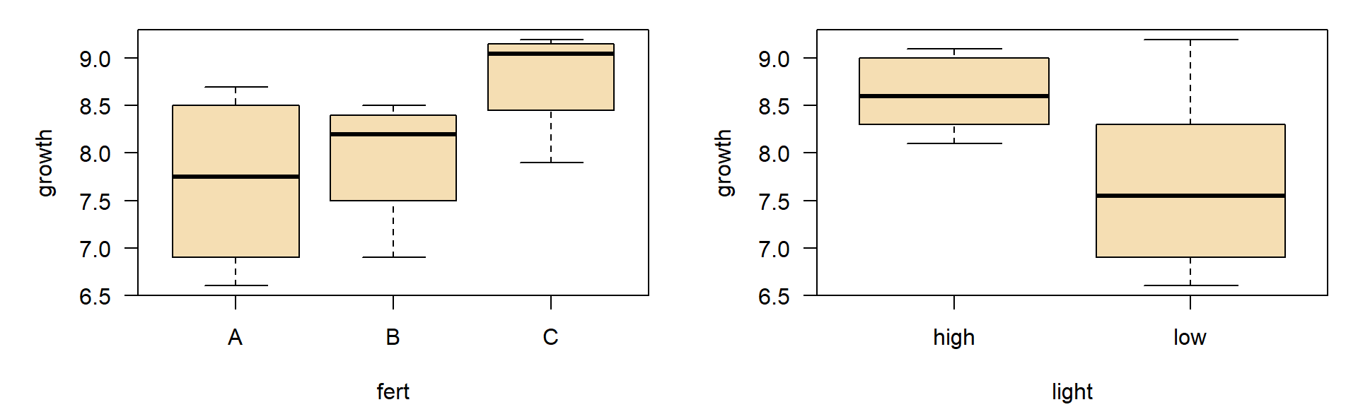
ANOVA

m <- lm(growth ~ light * fert, data = plants)
anova(m)

Analysis of Variance Table

Response: growth
           Df  Sum Sq Mean Sq F value  Pr(>F)  
light       1 2.61333 2.61333  7.2258 0.03614 *
fert        2 2.66000 1.33000  3.6774 0.09069 .
light:fert  2 0.68667 0.34333  0.9493 0.43833  
Residuals   6 2.17000 0.36167                  
---
Signif. codes:  0 '***' 0.001 '**' 0.01 '*' 0.05 '.' 0.1 ' ' 1

Interaction plot

with(plants, interaction.plot(fert, light, growth, 
                            col = c("orange", "brown"), lty = 1, lwd = 2))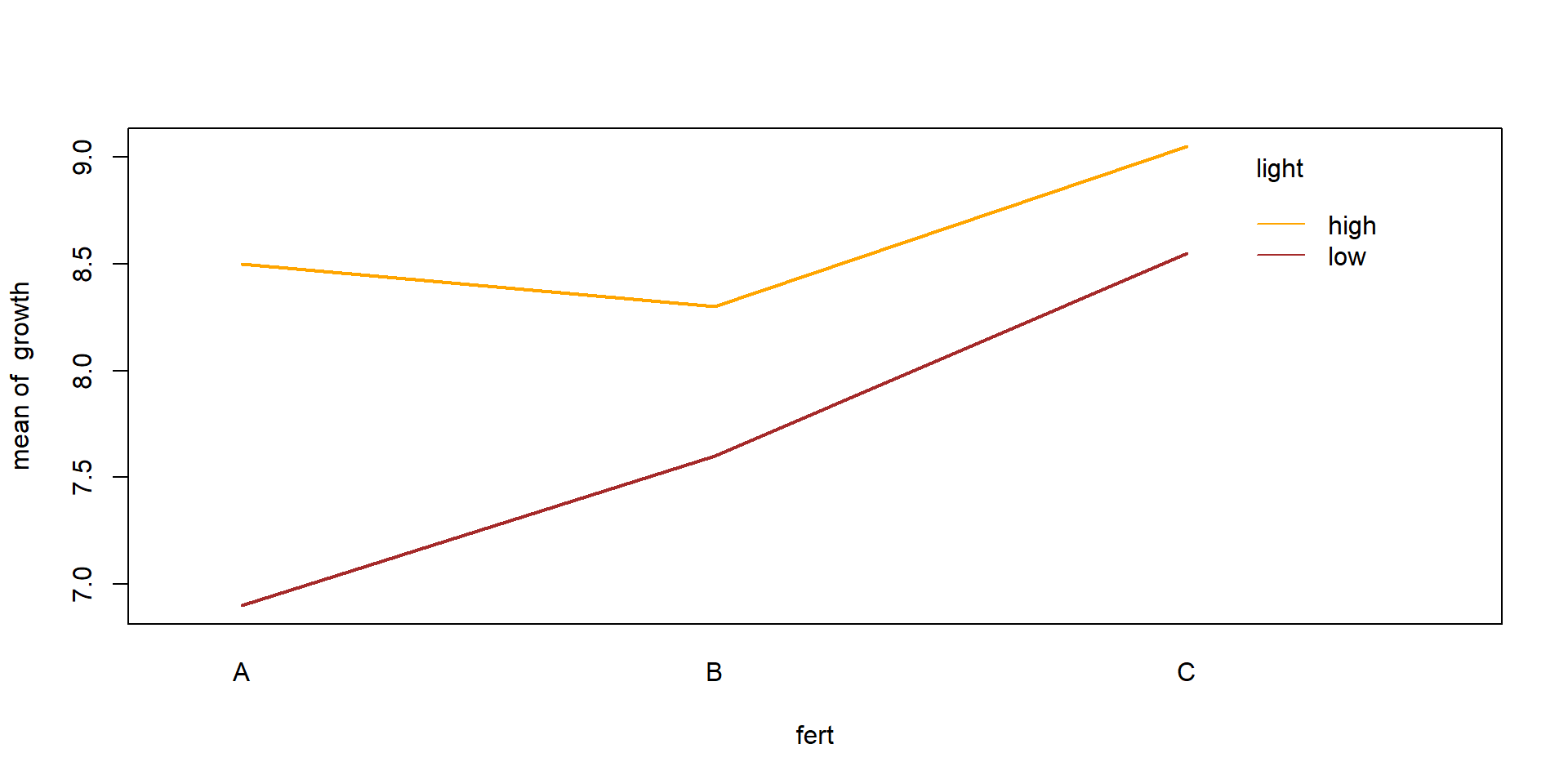

Diagnostics

Assumptions

1. Independence of measurements (within samples)
2. Variance homogeneity of residuals
3. Normal distribution of residuals

Test of assumptions needs residuals of the fitted model.

\(\Rightarrow\) Fit the ANOVA model first, then check if it was correct!

Diagnostic tools

• Box plot
• Plot of residuals vs. mean values
• Q-Q-plot of residuals
• Fligner-Killeen test (alternative: some people recommend the Levene-Test)

Diagnostics II

par(mfrow=c(1, 2))
par(cex=1.2, las=1)
qqnorm(residuals(m))
qqline(residuals(m))

plot(residuals(m)~fitted(m))
abline(h=0)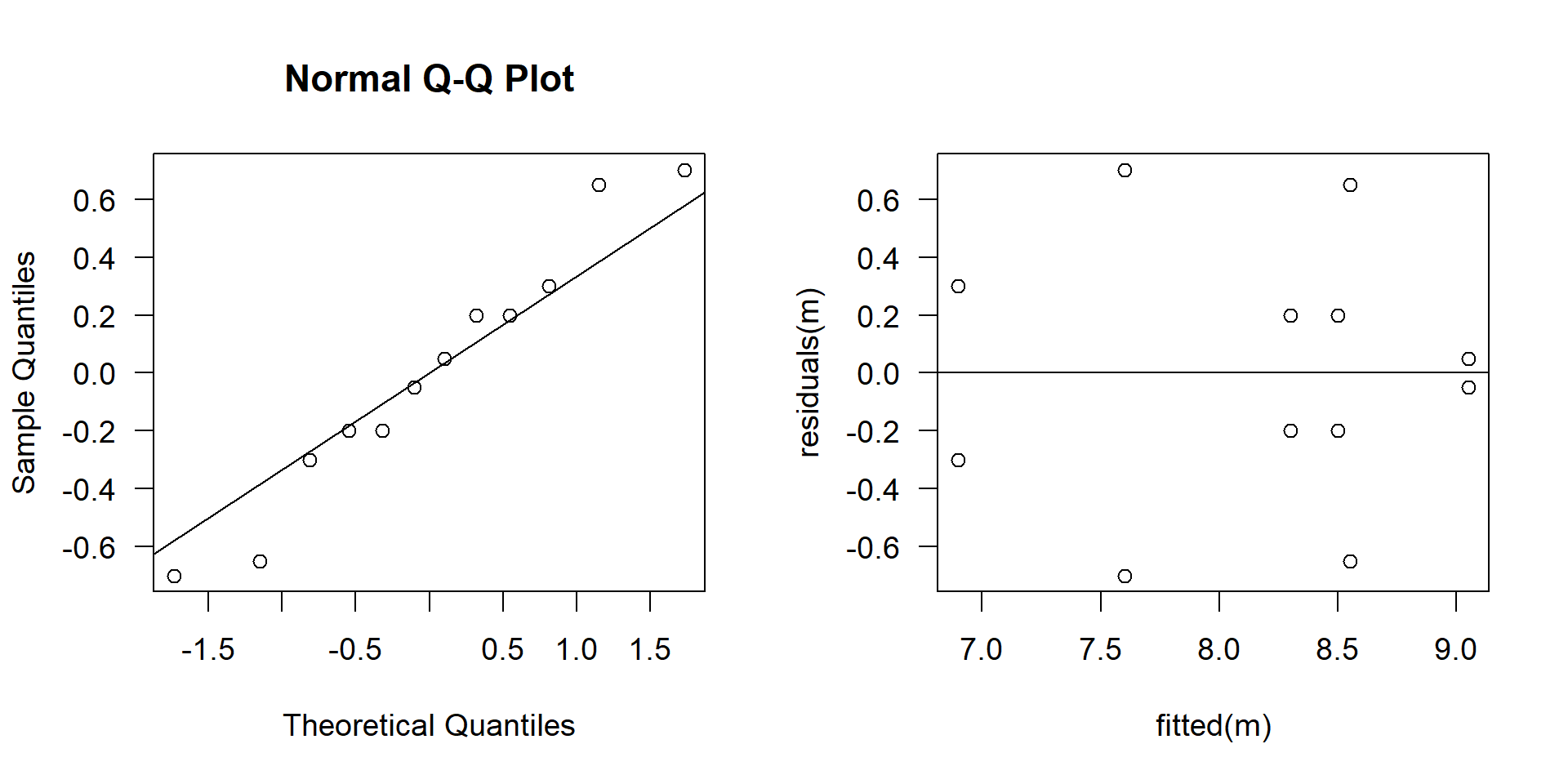

fligner.test(growth ~ interaction(light, fert), data=plants)

    Fligner-Killeen test of homogeneity of variances

data:  growth by interaction(light, fert)
Fligner-Killeen:med chi-squared = 10.788, df = 5, p-value = 0.05575

Residuals: look ok and p-value of the Fligner test \(> 0.05\), \(\rightarrow\) looks fine.

Notes

Linear regression or ANOVA?

• essentially the same
• independent variables are metric: linear model
• independent variables are nominal (= factor): ANOVA
• mix of metric and nominal variables: ANCOVA

Use of pre-tests

Pre-tests are in general questionable for theoretical reasons:

1. The null hypotheses \(H_0\) can only be rejected and not ultimately confirmed.
2. If the sample size is large, normality of residuals is not required
3. If \(p\) is close to the threshold and sample size is small, we would be left in uncertainty.

All this can only be overcome with careful thinking and some experience.

It is always a good idea to discuss results with colleagues and supervisors.

Sequential Holm-Bonferroni method

• Also called Holm procedure (Holm, 1979)
• Easy to use
• Can be applied to any multiple test problem
• Less conservative that ordinary Bonferroni correction, but …
• … still a very conservative approach
• see also Wikipedia

Algorithm

1. Select smallest \(p\) out of all \(n\) \(p\)-values
2. If \(p \cdot n < \alpha\) \(\Rightarrow\) significant, else STOP
3. Set \(n − 1 \rightarrow n\), remove smallest \(p\) from the list and go to step 1.

Example

Growth rate per day (\(d^{-1}\)) of blue-green algae cultures (Pseudanabaena) after adding toxic peptides from another blue-green algae (Microcystis).

The original hypothesis was that Microcystin LR (MCYST) or a derivative of it (Substance A) inhibits growth.

mcyst <-  data.frame(treat = factor(c(rep("Control", 5),
                                       rep("MCYST", 5),
                                       rep("Subst A", 5)),
                                levels=c("Control", "MCYST", "Subst A")),
                      mu   = c(0.086, 0.101, 0.086, 0.086, 0.099,
                               0.092, 0.088, 0.093, 0.088, 0.086,
                               0.095, 0.102, 0.106, 0.106, 0.106)
                     )

Approach 1: one-way ANOVA

par(mar=c(4, 8, 2, 1), las=1)
m <- lm(mu ~ treat, data=mcyst)
anova(m)

Analysis of Variance Table

Response: mu
          Df     Sum Sq    Mean Sq F value   Pr(>F)   
treat      2 0.00053293 2.6647e-04   8.775 0.004485 **
Residuals 12 0.00036440 3.0367e-05                    
---
Signif. codes:  0 '***' 0.001 '**' 0.01 '*' 0.05 '.' 0.1 ' ' 1

plot(TukeyHSD(aov(m)))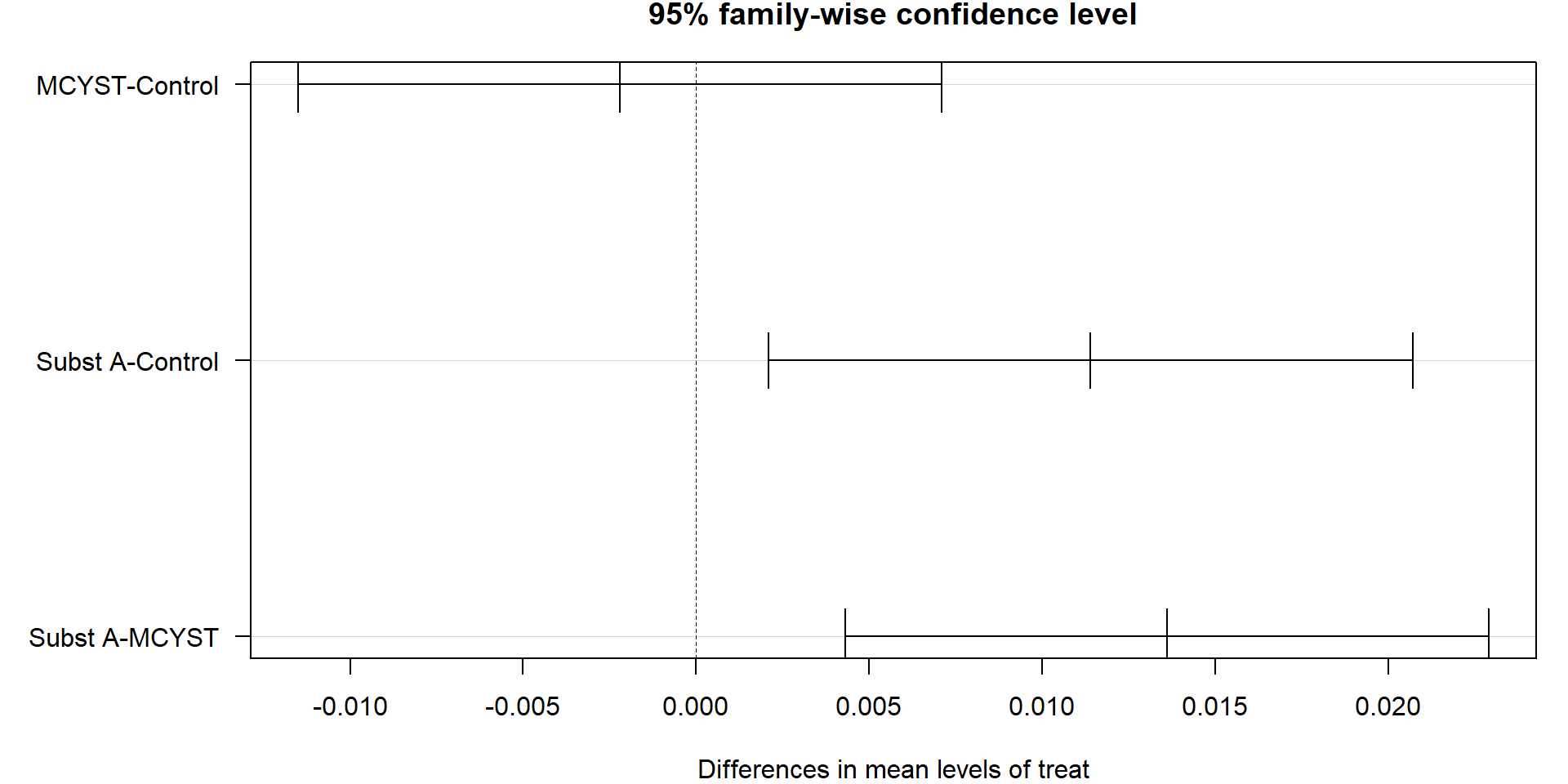

Approach 2: multiple t-tests with sequential Bonferroni correction

We separate the data set in single subsets:

Control <- mcyst$mu[mcyst$treat == "Control"]
MCYST   <- mcyst$mu[mcyst$treat == "MCYST"]
SubstA  <- mcyst$mu[mcyst$treat == "Subst A"]

and perform 3 t-Tests:

p1 <- t.test(Control, MCYST)$p.value
p2 <- t.test(Control, SubstA)$p.value
p3 <- t.test(MCYST, SubstA)$p.value

The following shows the raw p-values without correction:

c(p1, p2, p3)

[1] 0.576275261 0.027378832 0.001190592

… and with Holm correction:

p.adjust(c(p1, p2, p3))

[1] 0.576275261 0.054757664 0.003571775

Conclusions

Statistical methods

• In case of Holm-corrected t-tests, only a single p-value (MCYST vs. Subst A) remains significant. This indicates that in this case, Holm’s method is more conservative than TukeyHSD (only one compared to two significant) effects.
• An ANOVA with posthoc test is in general preferred,
• but the sequential Holm-Bonferroni can be helpful in special cases.
• Moreover, it demonstrates clearly that massive multiple testing needs to be avoided.

\(\Rightarrow\) ANOVA is to be preferred, when possible.

Interpretation

• Regarding our original hypothesis, we can see that MCYST and SubstA did not inhibit growth of Pseudanabaena. In fact SubstA stimulated growth.
• This was contrary to our expectations – the biological reason was then found 10 years later.

More about this can be found in Jähnichen et al. (2001), Jähnichen et al. (2007), Jähnichen et al. (2011), Zilliges et al. (2011) or Dziallas & Grossart (2011).

ANCOVA

Statistical question

• Comparison of regression lines
• Similar to ANOVA, but contains also metric variables (covariates)

Example

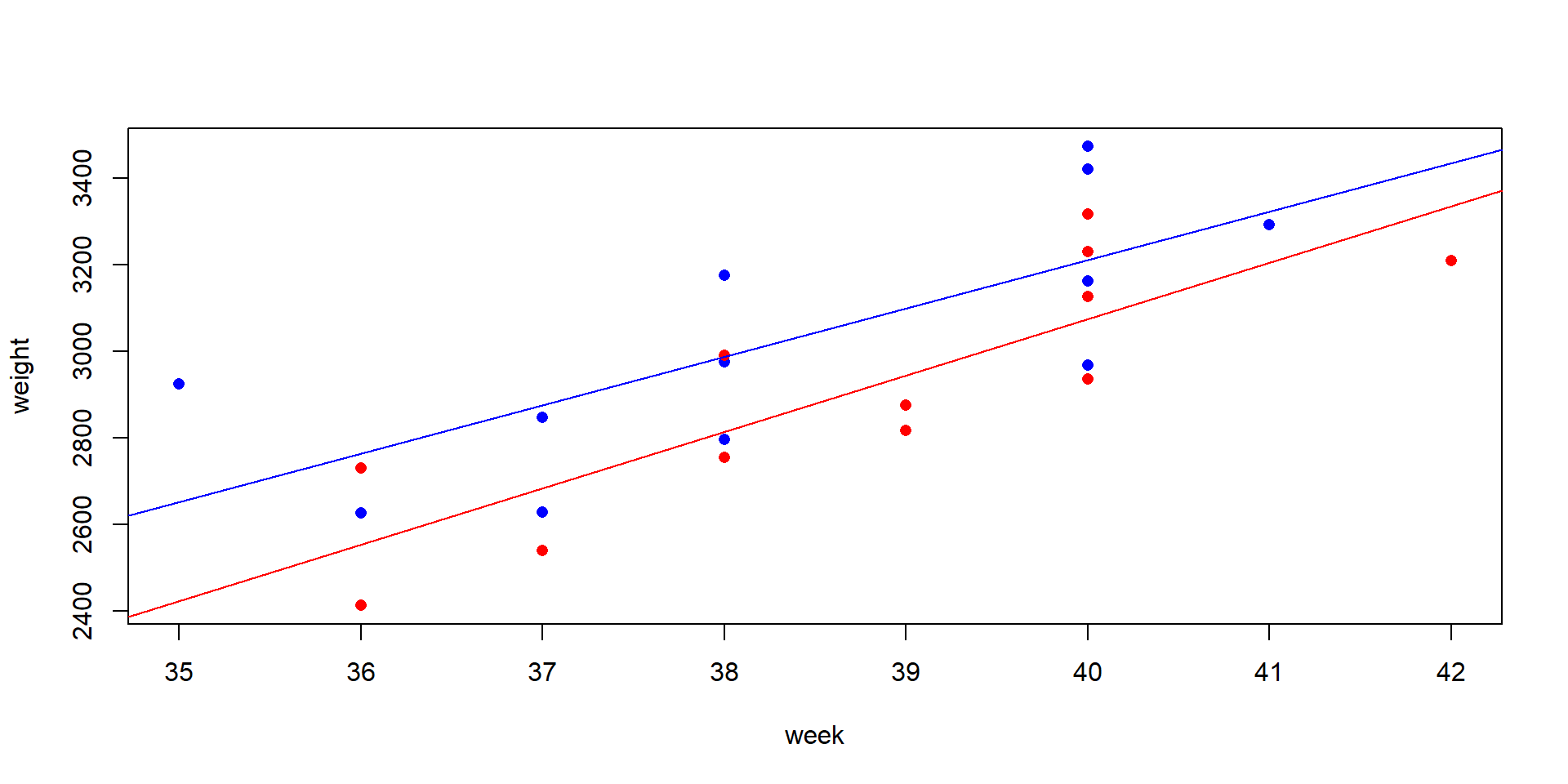
Annette Dobson’s birthweight data. A data set from a statistics textbook (Dobson, 2013), birth weight of boys and girls in dependence of the pregnancy week.

The birthweight data set

The data set is found at different places on the internet and in different versions.

Here the version that is found in an R demo: demo(lm.glm)

## Birth Weight Data see stats/demo/lm.glm.R
dobson <- data.frame(
  week = c(40, 38, 40, 35, 36, 37, 41, 40, 37, 38, 40, 38,
     40, 36, 40, 38, 42, 39, 40, 37, 36, 38, 39, 40),
  weight = c(2968, 2795, 3163, 2925, 2625, 2847, 3292, 3473, 2628, 3176,
        3421, 2975, 3317, 2729, 2935, 2754, 3210, 2817, 3126, 2539,
        2412, 2991, 2875, 3231),
  gender = gl(2, 12, labels=c("M", "F"))
)

Note: This is an artificial data set, not the reality.

Anette Dobson’s birthweight data

Why not just using a t-test?

boxplot(weight ~ gender,data = dobson, ylab = "weight")

t.test(weight ~ gender, data = dobson, var.equal = TRUE)

    Two Sample t-test

data:  weight by gender
t = 0.97747, df = 22, p-value = 0.339
alternative hypothesis: true difference in means between group M and group F is not equal to 0
95 percent confidence interval:
 -126.3753  351.7086
sample estimates:
mean in group M mean in group F 
       3024.000        2911.333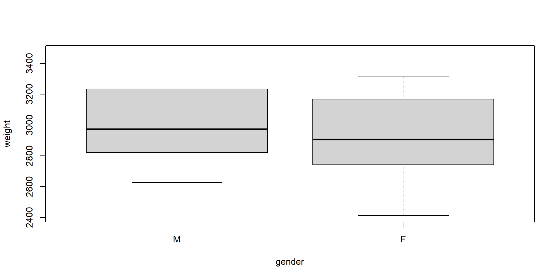 

The box plot shows much overlap and the difference is not significant, because the t-test ignores important information: the pregnancy week.

ANCOVA makes use of covariates

m <- lm(weight ~ week * gender, data = dobson)
anova(m)

Analysis of Variance Table

Response: weight
            Df  Sum Sq Mean Sq F value    Pr(>F)    
week         1 1013799 1013799 31.0779 1.862e-05 ***
gender       1  157304  157304  4.8221   0.04006 *  
week:gender  1    6346    6346  0.1945   0.66389    
Residuals   20  652425   32621                      
---
Signif. codes:  0 '***' 0.001 '**' 0.01 '*' 0.05 '.' 0.1 ' ' 1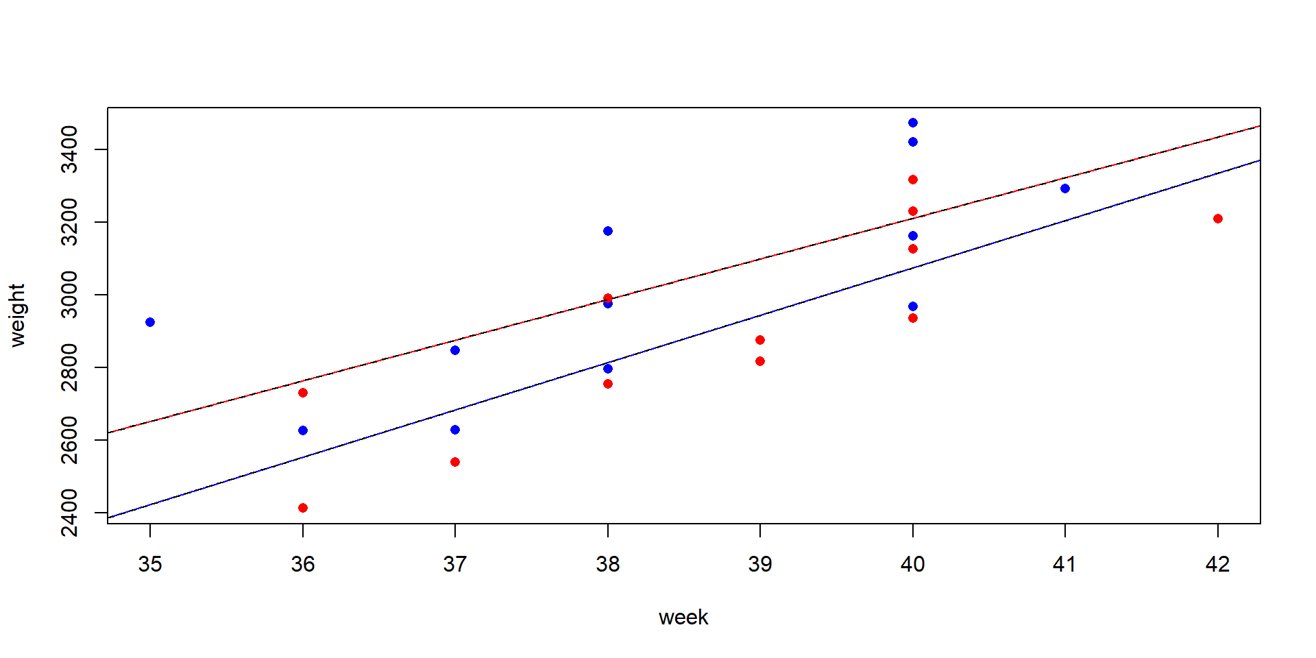

Pitfalls of ANOVA/ANCOVA

Pitfalls of ANOVA and ANCOVA described so far

1. Heterogeneity of variance
   • p-values can be biased (i.e. misleading or wrong)
   • use of a one-way ANOVA for uneaqual variances (in R: oneway.test)
2. Unbalanced case:
   unequal number of samples for each factor combination
   \(\rightarrow\) ANOVA results depend on the order of factors in the model formula.
   • Classical method: Type II or Type III ANOVA
   • Modern approach: model selection and likelihood ratio tests

Type II and type III ANOVA

• function Anova (with upper case A) in package car
• Help file of function Anova:

“Type-II tests are calculated according to the principle of marginality, testing each term after all others, except ignoring the term’s higher-order relatives; so-called type-III tests violate marginality, testing each term in the model after all of the others.”

• Conclusion: Use type II and not type III.
• Don’t try to interpret single terms in case of significant interactions.

Type II ANOVA: Example

library("car")
m <- lm(growth ~ light * fert, data = plants)
Anova(m, type="II")

Anova Table (Type II tests)

Response: growth
            Sum Sq Df F value  Pr(>F)  
light      2.61333  1  7.2258 0.03614 *
fert       2.66000  2  3.6774 0.09069 .
light:fert 0.68667  2  0.9493 0.43833  
Residuals  2.17000  6                  
---
Signif. codes:  0 '***' 0.001 '**' 0.01 '*' 0.05 '.' 0.1 ' ' 1

Model selection –
a paradigm change

Selection of an optimal model from a set of candidates

Problem:

• In complex ANOVA models, p-values depend on number (and sometimes of order) of included factors and interactions.
• The \(H_0\)-based approach becomes confusing, e.g. because of contradictory p-values.

Alternative approach:

• Employs the principle of parsimony

Instead of p-value based testing, comparison of different model candidates:

• Model with all potentiall effects → full model
• Omit single factors → reduced models (several!)
• No influence factors (ony mean value) → null model
• Which model is the best → minimal adequate model?

How can we measure which model is the best?

Compromise between model fit and model complexity (number of parameters, k).

• Goodness of fit: Likelihood L (measures how good the data match a given model).
• Log Likelihood: makes the criterion additive.
• AIC (Akaike Information Criterion):

\[AIC = −2 \ln(L) + 2k\]

• BIC (Bayesian Information Criterion), takes sample size into account (\(n\)):

\[BIC = −2 \ln(L) + k · \ln(n)\]

The model with the smallest AIC (or BIC) is the minimal adequate (i.e. optimal) model.

Model Selection and Likelihood Ratio Tests

Approach

1. Fit several models individually
2. Compare the models pairwise with ANOVA (likelihood ratio test)

Data and example

plants <- data.frame(No=1:12,
                   growth=c(6.6, 7.2, 6.9, 8.3, 7.9, 9.2,
                            8.3, 8.7, 8.1, 8.5, 9.1, 9.0),
                   fert= rep(c("A", "B", "C"), each=2),
                   light= rep(c("low", "high"), each=6)
                   )

m3 <- lm(growth ~ fert * light, data=plants)  # f1 + f2 + f1:f2
m2 <- lm(growth ~ fert + light, data=plants)  # f1 + f2
anova(m3, m2)

Analysis of Variance Table

Model 1: growth ~ fert * light
Model 2: growth ~ fert + light
  Res.Df    RSS Df Sum of Sq      F Pr(>F)
1      6 2.1700                           
2      8 2.8567 -2  -0.68667 0.9493 0.4383

• Likelihood ratio test compares two models (anova with > 1 model)
• Model with interaction (m3) not significantly better than model without interaction (m2).

AIC-based model selection

• pairwise model comparison is cumbersome, especially for large number of models.
• Solution: Create set of candidate models
• use smallest AIC to select the minimal adequate model.

m3  <- lm(growth ~ light * fert, data = plants) # full model
m2  <- lm(growth ~ light + fert, data = plants)
m1a <- lm(growth ~ fert, data = plants)
m1b <- lm(growth ~ light, data = plants)
m0  <- lm(growth ~ 1, data = plants)            # null model

AIC(m0, m1a, m1b, m2, m3)

    df      AIC
m0   2 33.38238
m1a  4 32.62699
m1b  3 30.72893
m2   5 26.83151
m3   7 27.53237

Note

• AIC values are defined up to an additive constant
• \(\rightarrow\) absolute values differ sometimes, depending on the applied method
• \(\Rightarrow\) look at range of AIC and differences, don’t care of absolute values
• rule of thumb: the “AIC unit” is 2, differences \(\approx 2.0\rightarrow\) minor importance

Stepwise model selection (automatic)

• The full model is supplied to the step function:

m1 <- lm(growth ~ fert * light, data=plants)
opt <- step(m1)

Start:  AIC=-8.52
growth ~ fert * light

             Df Sum of Sq    RSS     AIC
- fert:light  2   0.68667 2.8567 -9.2230
<none>                    2.1700 -8.5222

Step:  AIC=-9.22
growth ~ fert + light

        Df Sum of Sq    RSS     AIC
<none>               2.8567 -9.2230
- fert   2    2.6600 5.5167 -5.3256
- light  1    2.6133 5.4700 -3.4275

• Model with the smallest AIC
  \(\rightarrow\) optimal model.

anova(opt)

Analysis of Variance Table

Response: growth
          Df Sum Sq Mean Sq F value  Pr(>F)  
fert       2 2.6600 1.33000  3.7246 0.07190 .
light      1 2.6133 2.61333  7.3186 0.02685 *
Residuals  8 2.8567 0.35708                  
---
Signif. codes:  0 '***' 0.001 '**' 0.01 '*' 0.05 '.' 0.1 ' ' 1

• p < 0.05
  \(\rightarrow\) significant

Results of the example:

• optimal model (m2, opt), includes both factors fert and light but no interaction.
• \(\Rightarrow\) Model selection identified fert and light as necessary explanatory variables,
  in contrast to the classical ANOVA table where only light is significant.

Significance tests?

• The concept of model selection supercedes p-value-based statistics.
• Some authors generally discourage to use p-values in this context, others recommend a compromize.
• If you want to get a p-value, compare the optimal model with further reduced models, but still interpret the p-values with care:

anova(m2, m1a) # fert
anova(m2, m1b) # light

• In any case: focus on practical implications and don’t forget to report the effect sizes!

Summary of the ANOVA chapter

• Linear models form the basis of many statistical methods
  • Linear regression
  • ANOVA, ANCOVA, GLM, GAM, GLMM, . . .
  • ANOVA/ANCOVA instead of multiple testing
• ANOVA is more powerful than multiple tests:
  • avoids \(\alpha\)-error inflation
  • one big experiment needs less n than many small experiments
  • identification of interaction effects
  • elimination of co-variates
• Model selection vs. p-value based testing
  • paradigm shift in statistics: AIC instead of p-value
  • more reliable, especially for imbalanced or complex designs
  • extensible to generalized, additive, and mixed models (GLM, GAM, LME, GLMM, …)
  • but: p-value based tests are sometimes easier to understand

Avoid p-value hacking

Do NOT repeat experiments until a significant p-value is found.

The high-ranked journal “… Nature asked influential statisticians to recommend one change to improve science. The common theme? The problem is not our maths, but ourselves.” (Leek et al. (2017)):

Five ways to fix statistics. Comment on Nature

1. Jeff Leek: Adjust for human cognition
2. Blakeley B. McShane & Andrew Gelman: Abandon statistical significance
3. David Colquhoun: State false-positive risk, too
4. Michèle B. Nuijten: Share analysis plans and results
5. Steven N. Goodman: Change norms from within

Self study

Read the paper of Johnson & Omland (2004) to gain more understanding of the model selection paradigm.

Bibliography

Crawley, M. J. (2002). Statistical computing. An introduction to data analysis using S-PLUS (pp. 1–761). Wiley. datasets: http://www.bio.ic.ac.uk/research/mjcraw/statcomp/data/

Dobson, A. J. (2013). Introduction to statistical modelling. Springer.

Dziallas, C., & Grossart, H.-P. (2011). Increasing Oxygen Radicals and Water Temperature Select for Toxic Microcystis sp. PLoS ONE, 6(9), e25569. https://doi.org/10.1371/journal.pone.0025569

Holm, S. (1979). A simple sequentially rejective multiple test procedure. Scandinavian Journal of Statistics, 65–70. https://www.jstor.org/stable/4615733

Jähnichen, S., Ihle, T., Petzoldt, T., & Benndorf, J. (2007). Impact of Inorganic Carbon Availability on Microcystin Production by Microcystis aeruginosa PCC 7806. Applied and Environmental Microbiology, 73(21), 6994–7002. https://doi.org/10.1128/AEM.01253-07

Jähnichen, S., Long, B. M., & Petzoldt, T. (2011). Microcystin production by Microcystis aeruginosa: Direct regulation by multiple environmental factors. Harmful Algae, 12, 95–104. https://doi.org/10.1016/j.hal.2011.09.002

Jähnichen, S., Petzoldt, T., & Benndorf, J. (2001). Evidence for control of microcystin dynamics in Bautzen Reservoir (Germany) by cyanobacterial population growth rates and dissolved inorganic carbon. Fundamental and Applied Limnology, 150(2), 177–196. https://doi.org/10.1127/archiv-hydrobiol/150/2001/177

Johnson, G., Jerald, & Omland, K. S. (2004). Model Selection in Ecology and Evolution. Trends in Ecology and Evolution, 19(2), 101–108. https://doi.org/10.1016/j.tree.2003.10.013

Zilliges, Y., Kehr, J.-C., Meissner, S., Ishida, K., Mikkat, S., Hagemann, M., Kaplan, A., Börner, T., & Dittmann, E. (2011). The Cyanobacterial Hepatotoxin Microcystin Binds to Proteins and Increases the Fitness of Microcystis under Oxidative Stress Conditions. PLoS ONE, 6(3), e17615. https://doi.org/10.1371/journal.pone.0017615