06-Linear Regression

Applied Statistics – A Practical Course

Thomas Petzoldt

2024-11-14

Linear Regression

The linear model

\[ y_i = \alpha + \beta_1 x_{i,1} + \beta_2 x_{i,2} + \cdots + \beta_p x_{i,p} + \varepsilon_i \]

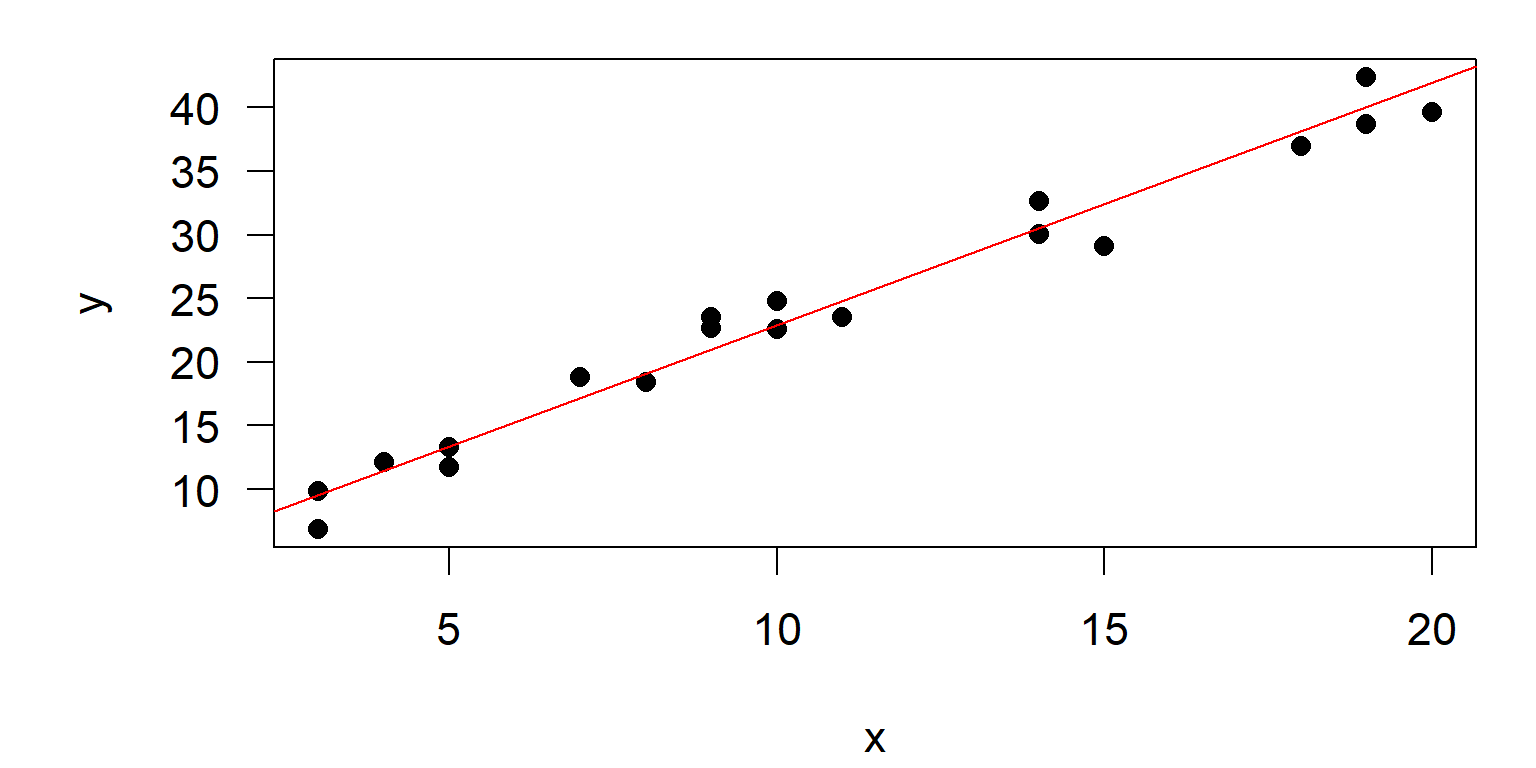
Fundamental for many statistical methods

• linear regression including some (at a first look) “nonlinear” functions
• ANOVA, ANCOVA, GLM (simultanaeous testing of multiple samples or multiple factors)
• multivariate statistics (e.g. PCA)
• time series analysis (e.g. ARIMA)
• imputation (estimation of missing values)

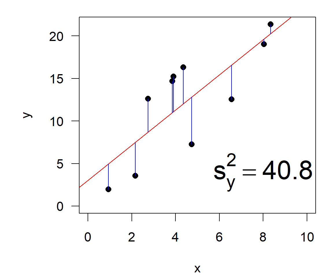
Method of least squares

\[ RSS = \sum_{i=1}^n (y_i - \hat{y}_i)^2 = \sum_{i=1}^n \varepsilon^2 \qquad \text{(residual sum of squares)} \]

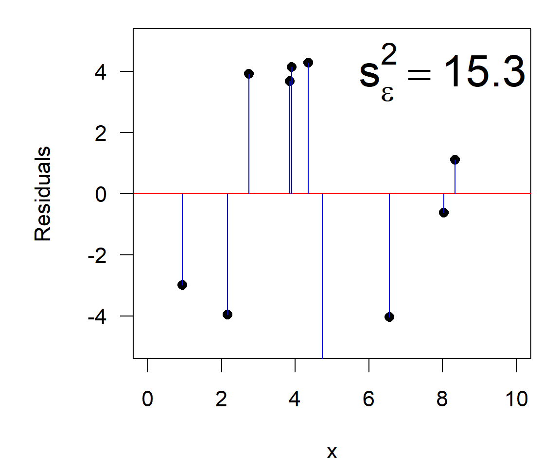
\[\begin{align} \text{total variance} &= \text{explained variance} &+& \text{residual variance}\\ s^2_y &= s^2_{y|x} &+& s^2_{\varepsilon} \end{align}\]

The coefficient of determination

\[\begin{align} r^2 & = \frac{\text{explained variance}}{\text{total variance}}\\ & = \frac{s^2_{y|x}}{s^2_y}\\ \end{align}\]

It can also be expressed as ratio of residual (RSS) and total (TSS) sum of squares:

\[ r^2 = 1-\frac{s^2_{\varepsilon}}{s^2_{y}} = 1-\frac{RSS}{TSS} = 1- \frac{\sum(y_i -\hat{y}_i)^2}{\sum(y_i - \bar{y})^2} \]

• derived from “sum of squares”, scaled as relative variance
• identical to the squared Pearson correlation \(r^2\) (in the linear case)
• very useful interpretation: percentage of variance of the raw data explained by the model

For the example: \(r^2= 1-\) 15.3 \(/\) 40.8 \(=\) 0.625

Minimization of RSS

• Analytical solution: minimize sum of squares (\(\sum \varepsilon^2\))
• Linear system of equations
• Minimum RSS \(\longleftarrow\) partial 1st derivatives (\(\partial\))

For \(y=a \cdot x + b\) with 2 parameters: \(\frac{\partial\sum \varepsilon^2}{\partial{a}}=0\), \(\frac{\partial\sum \varepsilon^2}{\partial{b}}=0\):

\[\begin{align} \frac{\partial \sum(\hat{y_i} - y_i)^2}{\partial a} &= \frac{\partial \sum(a + b \cdot x_i - y_i)^2}{\partial a} = 0\\ \frac{\partial \sum(\hat{y_i} - y_i)^2}{\partial b} &= \frac{\partial \sum(a + b \cdot x_i - y_i)^2}{\partial b} = 0 \end{align}\]

Solution of the linear system of equations:

\[\begin{align} b &=\frac {\sum x_iy_i - \frac{1}{n}(\sum x_i \sum y_i)} {\sum x_i^2 - \frac{1}{n}(\sum x_i)^2}\\ a &=\frac {\sum y_i - b \sum x_i}{n} \end{align}\]

• solution for arbitrary number of parameters with matrix algebra

Significance of the regression

\[ \hat{F}_{1;n-2;\alpha}= \frac{s^2_{explained}}{s^2_{residual}} = \frac{r^2(n-2)}{1-r^2} \]

Assumptions

1. Validity: the data maps to the research question
2. Additivity and linearity: \(y = \alpha + \beta_1 x_1 + \beta_2 x_2 + \cdots\)
3. Independence of errors: residuals around the regression line are independent
4. Equal variance of errors: residuals homogeneously distributed around the regression line
5. Normality of errors: the “assumption that is generally least important”

See: Gelman & Hill (2007) : Data analysis using regression …

Diagnostics

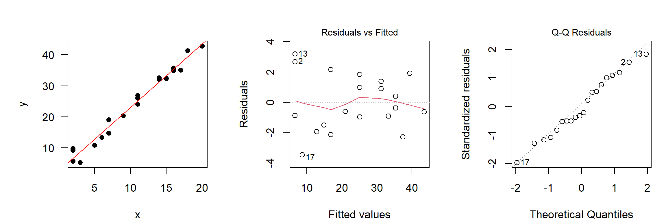
No regression analysis without graphical diagnostics!

• x-y-plot with regression line: is the variance homogeneous?
• Plot of residuals vs. fitted: are there still any remaining patterns?
• Q-Q-plot, histogram, : is distribution of residuals approximately normal?

Use graphical methods for normality, don’t trust the Shapiro-Wilks in that case.

Confidence intervals of the parameters

• based on standard errors and the t-distribution, similar to CI of the mean

\[\begin{align} a & \pm t_{1-\alpha/2, n-2} \cdot s_a\\ b & \pm t_{1-\alpha/2, n-2} \cdot s_b \end{align}\]

summary(m)

Call:
lm(formula = y ~ x)

Residuals:
    Min      1Q  Median      3Q     Max 
-3.4451 -1.0894 -0.4784  1.5065  3.1933 

Coefficients:
            Estimate Std. Error t value Pr(>|t|)    
(Intercept)  2.50740    0.87338   2.871   0.0102 *  
x            2.04890    0.07427  27.589 3.51e-16 ***
---
Signif. codes:  0 '***' 0.001 '**' 0.01 '*' 0.05 '.' 0.1 ' ' 1

Residual standard error: 1.885 on 18 degrees of freedom
Multiple R-squared:  0.9769,    Adjusted R-squared:  0.9756 
F-statistic: 761.1 on 1 and 18 DF,  p-value: 3.514e-16

Example: CI of a: \(a \pm t_{1-\alpha/2, n-2} \cdot s_a = 2.5074 \pm 2.09 \cdot 0.87338\)

Confidence interval and prediction interval

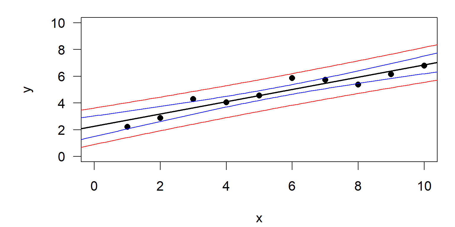
• Confidence interval:
  • Shows the area where the “true regression line” is expected by 95%.
  • Width of this band decreses with increasing \(n\)
  • analogous to the standard error
• Prediction interval:
  • Shows the range, in which the prediction for a single value is expected (by 95%).
  • Width is independent of sample size \(n\)
  • analogous to the standard deviation

Confidence intervals for linear regression: Code

## generate example data
x <- 1:10
y <- 2 + 0.5 * x + 0.5 * rnorm(x)

## fit model
reg <- lm(y ~ x)
summary(reg)

## plot data and regression line
plot(x,y, xlim = c(0, 10), ylim = c(0, 10), pch = 16)
abline(reg, lwd = 2)

## calcuate and plot intervals
newdata <- data.frame(x=seq(-1, 11, length=100))
conflim <- predict(reg, newdata=newdata, interval = "confidence")
predlim <- predict(reg, newdata=newdata, interval = "prediction")

lines(newdata$x, conflim[,2], col = "blue")
lines(newdata$x, conflim[,3], col = "blue")
lines(newdata$x, predlim[,2], col = "red")
lines(newdata$x, predlim[,3], col = "red")

• The variable newdata:
  • spans the range of x values in small steps to get a smooth curve
  • single column with exactly the same name x as in the model formula
  • for multiple regression, one column per explanation variable

Problematic cases

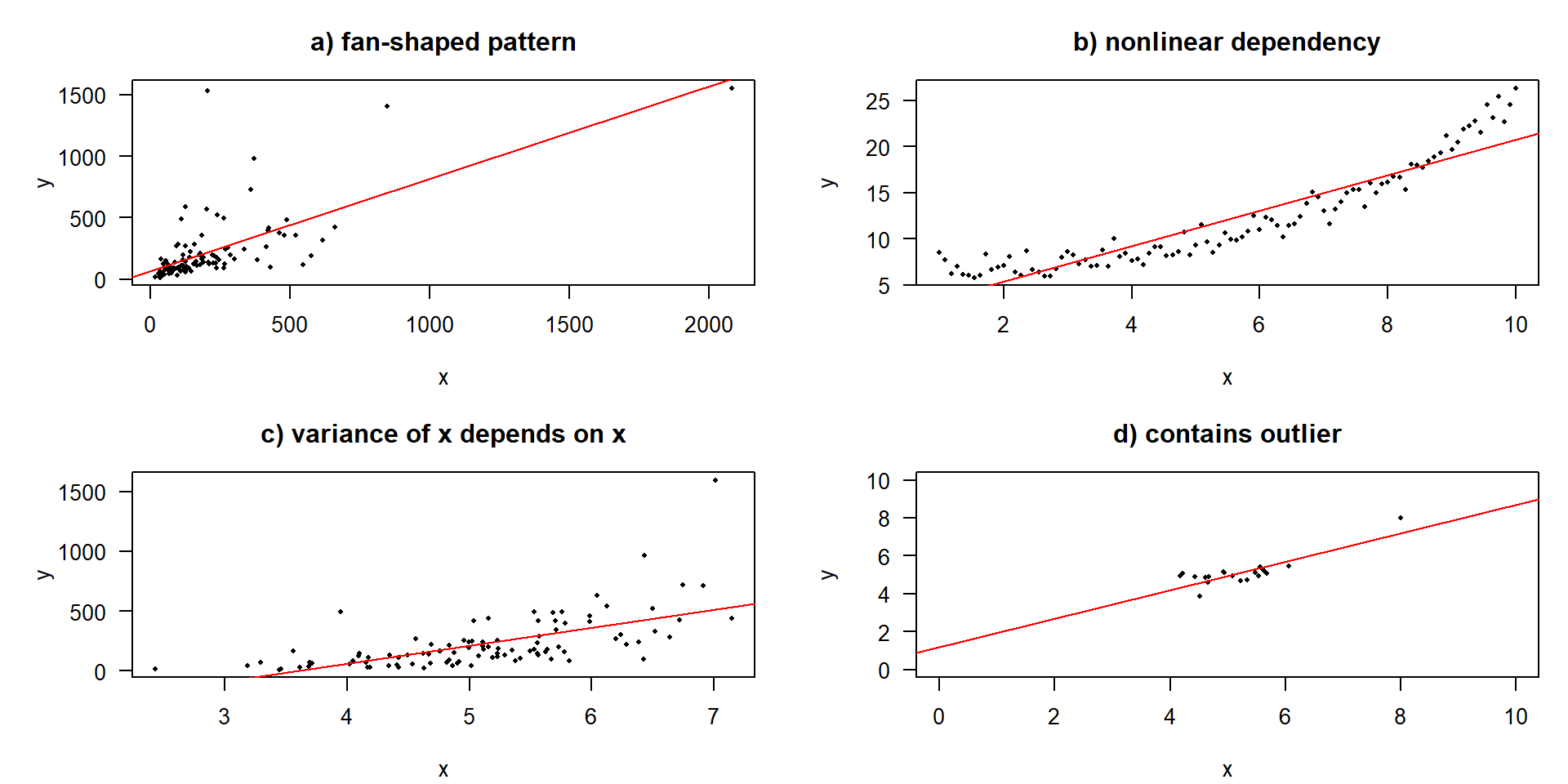
Identification and treatment of problematic cases

Rainbow-Test (linearity)

## generate test data
x <- 1:10
y <- 2 + 0.5 * x + 0.5 * rnorm(x)

library(lmtest)
raintest(y~x)

    Rainbow test

data:  y ~ x
Rain = 0.79952, df1 = 5, df2 = 3, p-value = 0.6153

Breusch-Pagan-test (variance homogeneity)

bptest(y~x)

    studentized Breusch-Pagan test

data:  y ~ x
BP = 3.3989, df = 1, p-value = 0.06524

Non-normality and outliers

• Non-normality
  • less important than many people think (due to the CLT)
  • transformations (e.g. Box-Cox), polynomials, periodic functions
  • use of GLM’s (generalized linear models)

• Outliers (depends on pattern)
  • use of transformations (e.g. double log)
  • use of outlier-tests, e.g. outlierTest from package car
  • robust regression with IWLS (iteratively re-weighted least squares) from package MASS

Robust regression with IWLS

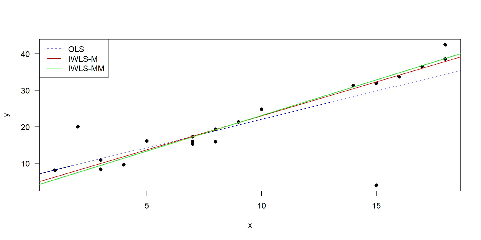
• IWLS: iterated re-weighted least squares
• OLS (ordinary least squares) is “normal” linear regression
• M-estimation and MM-estimation are two different approaches, details in Venables & Ripley (2013)
• robust regression is preferred over outlier exclusion

Code of the IWLS regression

library("MASS")

## test data with 2 "outliers"
x <- c(1, 2, 3, 3, 4, 5, 7, 7, 7, 8, 8, 9, 10, 14, 15, 15, 16, 17, 18, 18)
y <- c(8.1, 20, 10.9, 8.4, 9.6, 16.1, 17.3, 15.3, 16, 15.9, 19.3, 
       21.3, 24.8, 31.3, 4, 31.9, 33.7, 36.5, 42.4, 38.5)

## fit the models
ssq    <- lm(y ~ x)
iwls   <- rlm(y ~ x)
iwlsmm <- rlm(y ~ x, method = "MM")

## plot the models
plot(x, y, pch = 16, las = 1)
abline(ssq, col = "blue", lty = "dashed")
abline(iwls, col = "red")
abline(iwlsmm, col = "green")
legend("topleft", c("OLS", "IWLS-M", "IWLS-MM"),
       col = c("blue", "red", "green"),
       lty = c("dashed", "solid", "solid"))

Further reading

• Kleiber & Zeileis (2008) Applied econometrics with R. Springer Verlag.
• Venables & Ripley (2013) Modern applied statistics with S-PLUS (3rd ed.). Springer Science & Business Media.
• Fox & Weisberg (2018) An R companion to applied regression. Sage publications.
• Gelman & Hill (2007) Data analysis using regression and multilevel hierarchical models (Vol. 1). Cambridge University Press, New York.

References

Fox, J., & Weisberg, S. (2018). An R companion to applied regression. Sage publications.

Gelman, A., & Hill, J. (2007). Data analysis using regression and multilevelhierarchical models (Vol. 1). Cambridge University Press New York, NY, USA.

Kleiber, C., & Zeileis, A. (2008). Applied econometrics with R. Springer.

Venables, W. N., & Ripley, B. D. (2013). Modern applied statistics with S-PLUS (3rd ed.). Springer Science; Business Media.