A statistical hypothesis test is a method of statistical inference.
Commonly, two samples are compared, or a sample is compared against properties from an idealized model.
A hypothesis \(H_a\) for the statistical relationship between the two data sets, is compared to an idealized null hypothesis \(H_0\) that proposes no relationship between two data sets.
The comparison is considered statistically significant if the relationship between the data sets would be an unlikely realization of the null hypothesis according to a threshold probability – the significance level.
relative effect size \(\delta\) (also called Cohen’s d)
significance means that an observed effect is unlikely the result of pure random variation.
Null hypothesis and alternative hypothesis
\(H_0\) null hypothesis: two populations are not different with respect to a certain property.
Assumption: observed effect occured purely at random, true effect is zero.
\(H_a\) alternative hypothesis (experimental hypothesis): existence of a certain effect.
An alternative hypothesis is never completely true or “proven”.
Acceptance of \(H_A\) means only than \(H_0\) is unlikely.
“Not significant” means either no effect or sample size too small!
Note: Different meaning of significance (\(H_0\) unlikely) and relevance (effect large enough to play a role in practice).
The p-value
The interpretation of the p-value was often confused in the past, even in statistics textbooks, so it is good to refer to a clear definition:
The p-value is defined as the probability of obtaining a result equal to or ‘more extreme’ than what was actually observed, when the null hypothesis is true.
Hubbard (2004) Alphabet Soup: Blurring the Distinctions Between p’s and a’s in Psychological Research, Theory Psychology 14(3), 295-327. DOI: 10.1177/0959354304043638
Alpha and beta errors
Reality
Decision of the test
correct?
probability
\(H_0\) = true
significant
no
\(\alpha\)-error
\(H_0\) = false
not significant
no
\(\beta\)-error
\(H_0\) = true
not significant
yes
\(1-\alpha\)
\(H_0\) = false
significant
yes
\(1-\beta\) (power)
1.\(H_0\) falsely rejected (error of the first kind or \(\alpha\)-error)
we claim an effect, that does not exist, e.g. a drug with no effect
2.\(H_0\) falsely retained (error of the second kind or \(\beta\)-error)
typical case in small studies, where effect was not enough to detect existing effects
Use in practice
common convention in environmental sciences: \(\alpha=0.05\), must be set beforehand
\(\beta=f(\alpha, \text{effectsize}, \text{sample size}, \text{kind of test})\), should be \(\le 0.2\)
Significance and relevance
Significance is not the only important. Focus also on effect size and relevance!
Statistical significance means that the null hypothesis \(H_0\) is unlikely in a statistical sense.
Practical relevance (sometimes called “practical significance”) means that the effect size is large enough to play a role in practice.
This means that whether an effect can be relevant or not depends on its effect size and the field of application.
Let’s for example consider a vaccination. If a vaccine had a significant effect in a clinical test, but protected only 10 out of 1000 people, one would not consider this effect as relevant and not produce this vaccine.
On the other hand, even small effects can be relevant. So if a toxic substance would have an effect on 1 out of 1000 people to produce cancer, we would consider this as relevant. To detect this as a significant effect would need an epidemiological study with a large number of people. But as it is highly relevant, it is worth the effort.
Take home messages
A p-value measures the probability that a purely random effect would be equally or more extreme than an observed effect if the null hypothesis is true.
Significant means the results are unlikely if there were no real effect.
Not significant doesn’t mean “no effect”.
Non-significant results suggest the need for further research, e.g.:
increase sample size
increase experimental effect
reduce experimental error
consider a more powerful statistical procedure
Don’t focus on p-values alone. Never forget to report also sample size, effect size and relevance of your results.
With large datasets:
statistically significant results can easily be obtained even for very small and practically irrelevant effects.
\(\rightarrow\) effect size and relevance become more important than p-values.
The p-value remains an important tool in statistics, but misuse can lead to misinterpretation.
Differences between mean values
One sample t-Test
tests if a sample is from a population with given mean value \(\mu\)
based on checking if the population mean \(\mu\) is in the confidence interval of \(\bar{x}\)
Let’s assume a sample of size with \(n=10, \bar{x}=5.5, s=1\) and \(\mu=5\).
Estimate the 95% confidence interval of \(\bar{x}\):
\[
CI = \bar{x} \pm t_{1-\alpha/2, n-1} \cdot s_{\bar{x}}
\] with \[
s_{\bar{x}} = \frac{s}{\sqrt{n}} \qquad \text{(standard error)}
\]
Different ways of calculation shown at the next slides
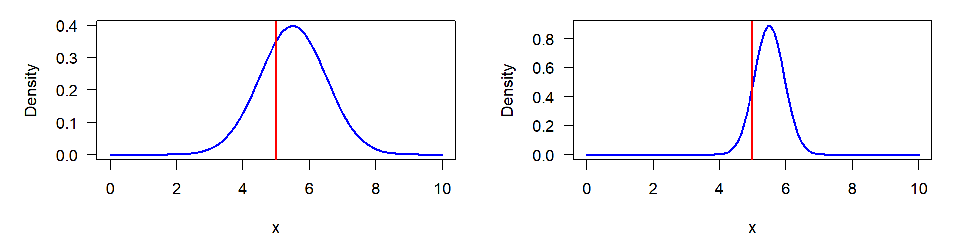
Remember: standard deviation and standard error
Visualization of a one-sample t-test. Left: original distribution of the data measured by standard deviation, right: distribution of mean values, measured by its standard error.
    One Sample t-test

data:  x
t = 1.5811, df = 9, p-value = 0.1483
alternative hypothesis: true mean is not equal to 5
95 percent confidence interval:
 4.784643 6.215357
sample estimates:
mean of x
      5.5
The test returns the observed t-value, the 95% confidence interval and the p-value.
An important difference is, that this method needs the original data, while the other methods need only mean, standard deviation and sample size.
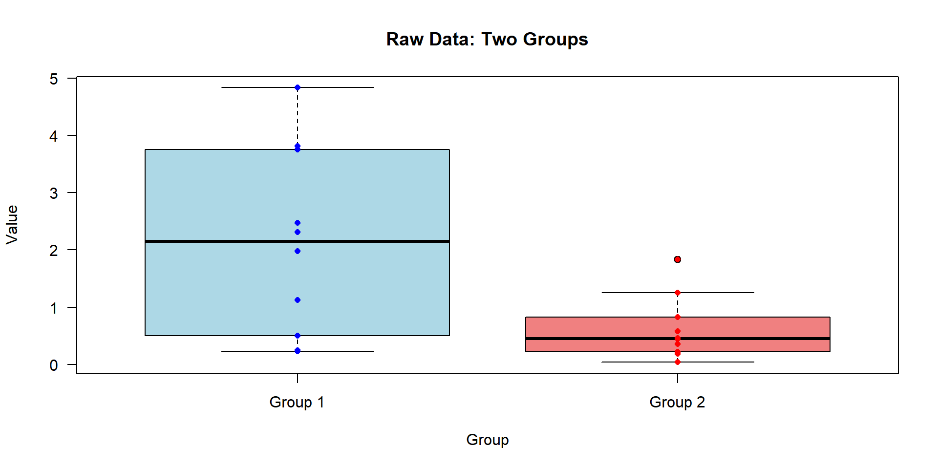
Two sample t-test
The two-sample t-test compares two independent samples:
    Welch Two Sample t-test

data:  x1 and x2
t = -3.7185, df = 21.611, p-value = 0.001224
alternative hypothesis: true difference in means is not equal to 0
95 percent confidence interval:
 -2.3504462 -0.6662205
sample estimates:
mean of x mean of y
 5.475000  6.983333
\(\rightarrow\) both samples differ significantly (\(p < 0.05\))
Note: R has not performed the “ordinary” t-test but the Welch test (= heteroscedastic t-test)
where variances of both samples don’t need to be identical.
    Welch Two Sample t-test

data:  x1 and x2
t = -3.7185, df = 21.611, p-value = 0.001224
alternative hypothesis: true difference in means is not equal to 0
95 percent confidence interval:
 -2.3504462 -0.6662205
sample estimates:
mean of x mean of y
 5.475000  6.983333
… is just the default method of the t.test-function.
Equality of variance: F-test
\(H_0\): \(\sigma_1^2 = \sigma_2^2\)
\(H_a\): variances unequal
Test criterion:
\[F = \frac{s_1^2}{s_2^2} \]
larger of the two variances in the enumerator \((s^2_1 > s^2_2)\)
    Two Sample t-test

data:  x1 and x2
t = -1.372, df = 8, p-value = 0.2073
alternative hypothesis: true difference in means is not equal to 0
95 percent confidence interval:
 -4.28924  1.08924
sample estimates:
mean of x mean of y
      4.0       5.6
    Paired t-test

data:  x1 and x2
t = -4, df = 4, p-value = 0.01613
alternative hypothesis: true mean difference is not equal to 0
95 percent confidence interval:
 -2.710578 -0.489422
sample estimates:
mean difference
           -1.6
p=0.016, significant
It can be seen that the paired t-test has a greater discriminatory power in this case.
Mann-Whitney and Wilcoxon-test
Non-parametric tests:
No assumptions about shape and parameters of distribution, but
distributions should be similar, otherwise test may be misleading.
Based on Ranks: Tests compare the ranks of the data.
Use Mann-Whitney for independent samples, Wilcoxon for paired samples.
Basic principle: Count of so-called “inversions” of ranks, where samples overlap
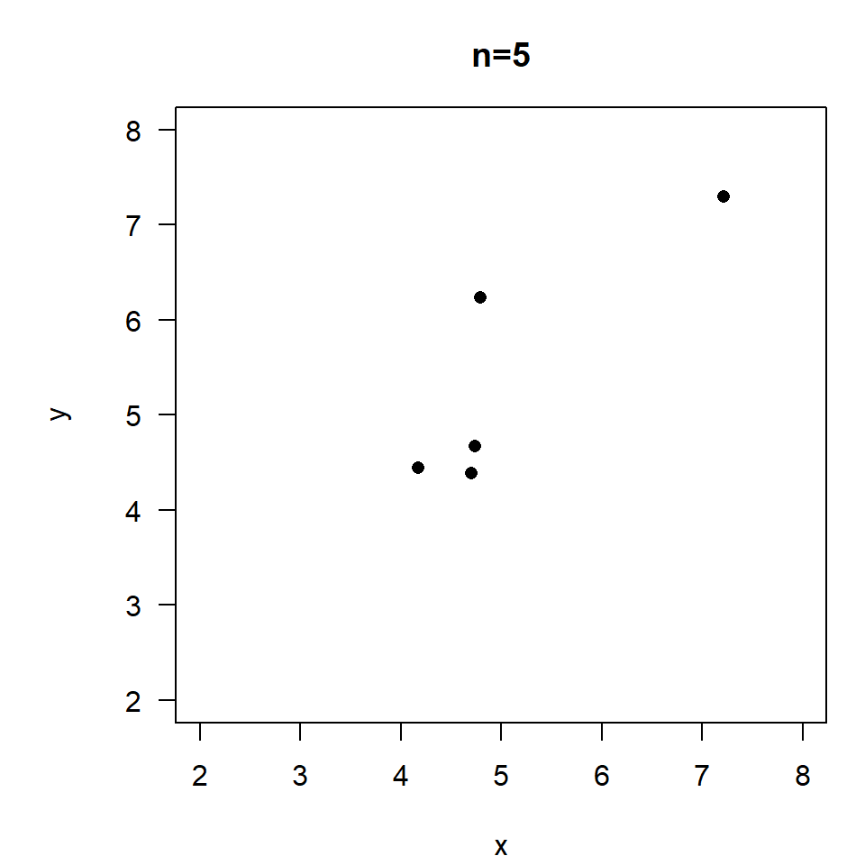
The power of a t-test, or the minimum sample size, can be calculated with: power.t.test():
power.t.test(n=5, delta=0.5, sig.level=0.05)
     Two-sample t test power calculation

              n = 5
          delta = 0.5
             sd = 1
      sig.level = 0.05
          power = 0.1038399
    alternative = two.sided

NOTE: n is number in *each* group
\(\rightarrow\) power = 0.10
For \(n=5\) an existing effect of \(0.5\sigma\) is only detected in 1 out of 10 cases.
For a power of 80% at \(n=5\) we need an effect size of at least \(2\sigma\):
power.t.test(n=5, power=0.8, sig.level=0.05)
For a weak effect of \(0.5\sigma\) we need a sample size of \(n\ge64\) in each group:
power.t.test(delta=0.5,power=0.8,sig.level=0.05)
\(\Rightarrow\) we need either a large sample size or a strong effect.
Simulated power of a t-test
# population parametersn <-10xmean1 <-50; xmean2 <-55xsd1 <- xsd2 <-10alpha <-0.05nn <-1000# number of test runs in the simulationa <- b <-0# initialize countersfor (i in1:nn) {# create random numbers x1 <-rnorm(n, xmean1, xsd1) x2 <-rnorm(n, xmean2, xsd2)# results of the t-test p <-t.test(x1,x2,var.equal =TRUE)$p.value if (p < alpha) { a <- a+1 } else { b <- b+1 }}print(paste("a=", a, ", b=", b, ", a/n=", a/nn, ", b/n=", b/nn))
Test for distributions
Testing for distributions
Nominal variables
\(\chi^2\)-test
Fisher’s exact test
Ordinal variables
Cramér-von-Mises-Test
\(\rightarrow\) more powerful than \(\chi^2\) or KS-test
Metric scales
Kolmogorov-Smirnov-Test (KS-test)
Shapiro-Wilks-Test (for normal distribution)
Graphical checks
Contingency tables for nominal variables
used for nominal (i.e. categorical or qualitative) data
examples: eye and hair color, medical treatment and the number of cured/not cured
important: use absolute mesurements (true numbers!), not percentages or other calculated data (e.g. not something like biomass per area)
Example: Occurence of Daphnia (water flea) in a lake:
Clone
Upper layer
Deep layer
A
50
87
B
37
78
C
72
45
food algae in the deep water, that was poor of oxygen
genetically evolved clones with higher haemoglobin content can dive into deep water
    Chi-squared test for given probabilities with simulated p-value (based
    on 1000 replicates)

data:  obsfreq
X-squared = 13.647, df = NA, p-value = 0.0959
one-sample\(\chi^2\)-test. It tests for equality of frequency in all classes.
The simulation-based version of the test (with 1000 replicates) is slightly more precise than the standard \(\chi^2\)-test, but both are not significant.
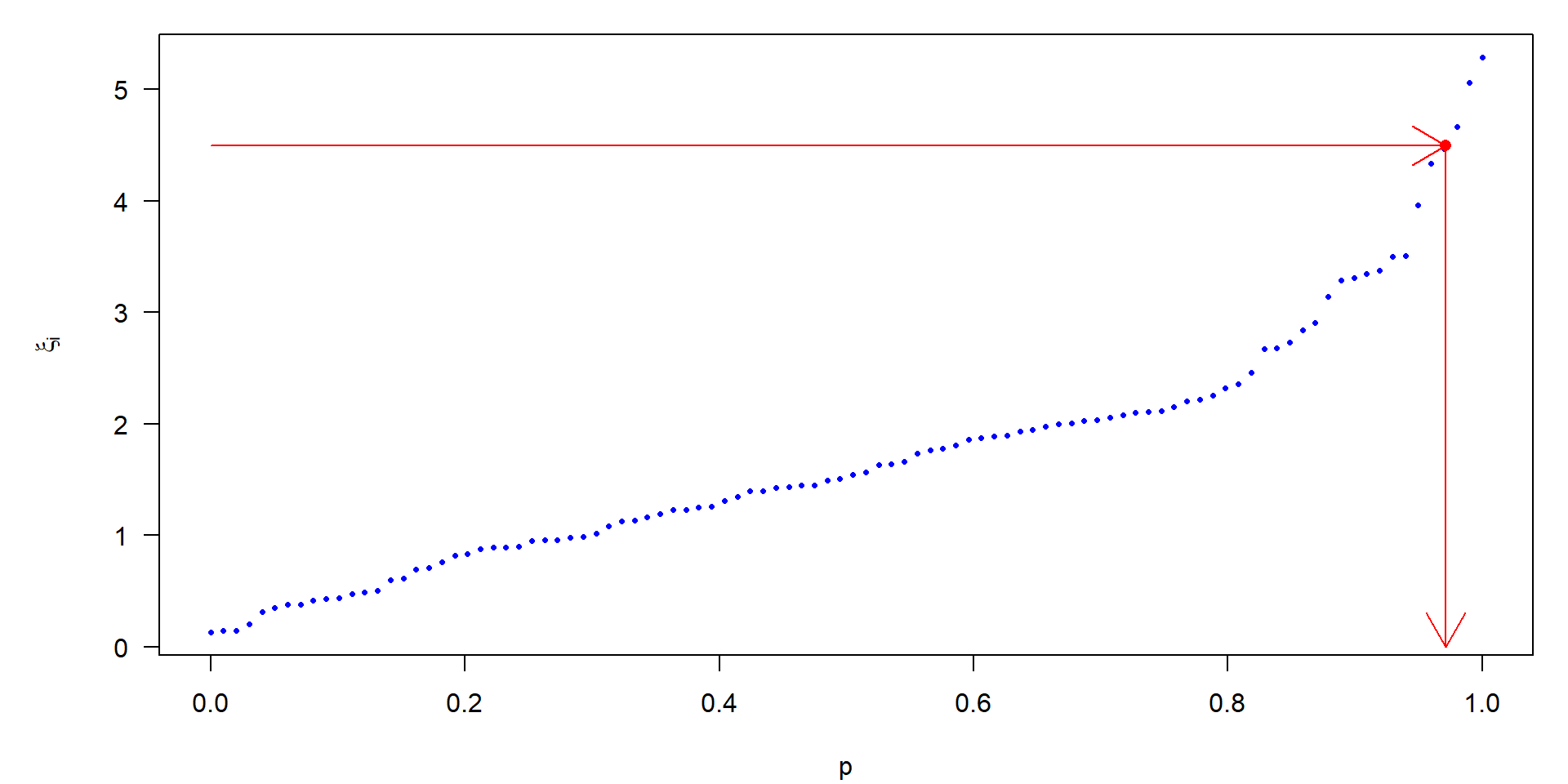
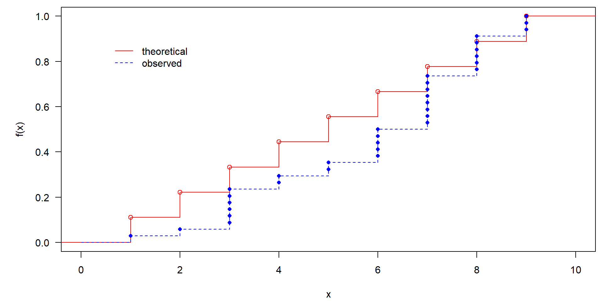
Cramér-von-Mises-Test
\[
T = n \omega^2 = \frac{1}{12n} + \sum_{i=1}^n \left[ \frac{2i-1}{2n}-F(x_i) \right]^2
\]
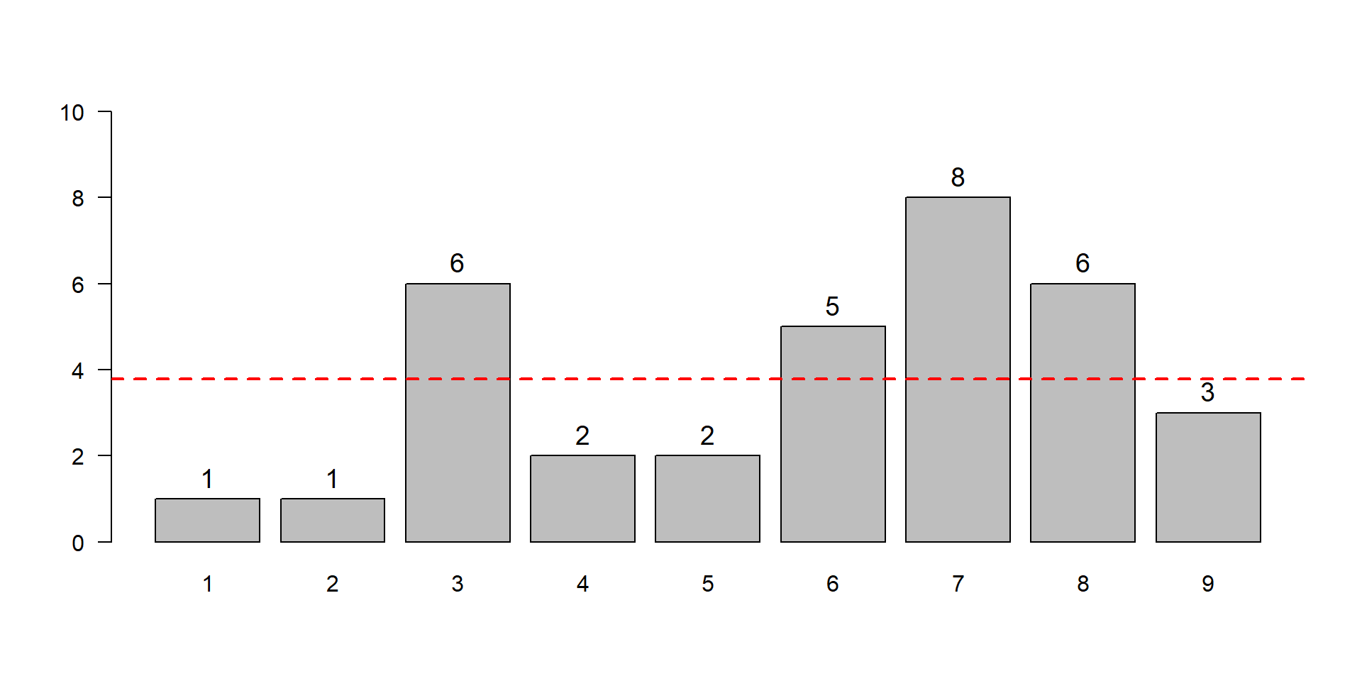
Cramér-von-Mises-Test in R
library(dgof)obsfreq <-c(1, 1, 6, 2, 2, 5, 8, 6, 3)## CvM-test needs individual values, not class frequenciesx <-rep(1:length(obsfreq), obsfreq)x
## create a cumulative function with equal probability of all casescdf <-stepfun(1:9, cumsum(c(0, rep(1/9, 9))))cdf <-ecdf(1:9)## perform the testcvm.test(x, cdf)
    Cramer-von Mises - W2

data:  x
W2 = 0.51658, p-value = 0.03665
alternative hypothesis: Two.sided
The Cramér-von-Mises-test works with the original, unbinned values
Use of cumulative distribution function respects order of classes\(\rightarrow\) more powerful, than \(\chi^2\)-test.
Testing for normal distribution
Why do we want this?
Sometimes we want to know whether a data set belongs to a specific type of distribution. Though this sounds easy, it appears quite difficult for theoretical reasons:
statistical tests check for deviations from the null hypothesis
but here we want to test the opposite, if \(H_0\) is true
This is in fact impossible, because “not significant” means only that a potential effect is either not existent or just too small to be detected. On the opposite, “significantly different” includes a certain probability of false positives.
However, most statistical tests do not require perfect agreement with a certain distribution:
t-test and ANOVA assume normality of residuals
due to the CLT, the distribution of sums and mean values converges to normal
Testing or checking?
Philosophical problem: We want to keep the \(H_0\)!
Equality cannot be tested
Therefore: better to say “checking normality”.
Think first
Does normal distribution “makes sense” for the data?
Are the data metric (continuous)?
What is the data generating process? \(\rightarrow\) Contextual understanding!
Inherent non-normality
Some types of data, such as count data (e.g., number of occurrences) and binary data (e.g., yes/no), are inherently non-normal.
Binary data: use methods for Binomial distribution with raw data instead of percentages
Count data: use methods designed for Poisson distribution
Shapiro-Wilks-W-Test ?
\(\rightarrow\) Aim: tests if a sample conforms to a normal distribution
x <-runif(20)shapiro.test(x)
    Shapiro-Wilk normality test

data:  x
W = 0.93541, p-value = 0.1961
\(\rightarrow\) the \(p\)-value is greater than 0.05, so we would keep \(H_0\) and conclude that nothing speaks against acceptance of the normal
Interpration of the Shapiro-Wilks-test needs to be done with care:
for small \(n\), the test is not sensitive enough
far large \(n\), it is over-sensitive
using Shapiro-Wilks to check normality for t-test and ANOVA is not anymore recommended
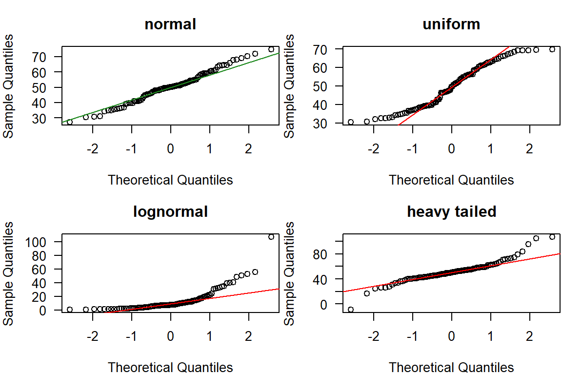
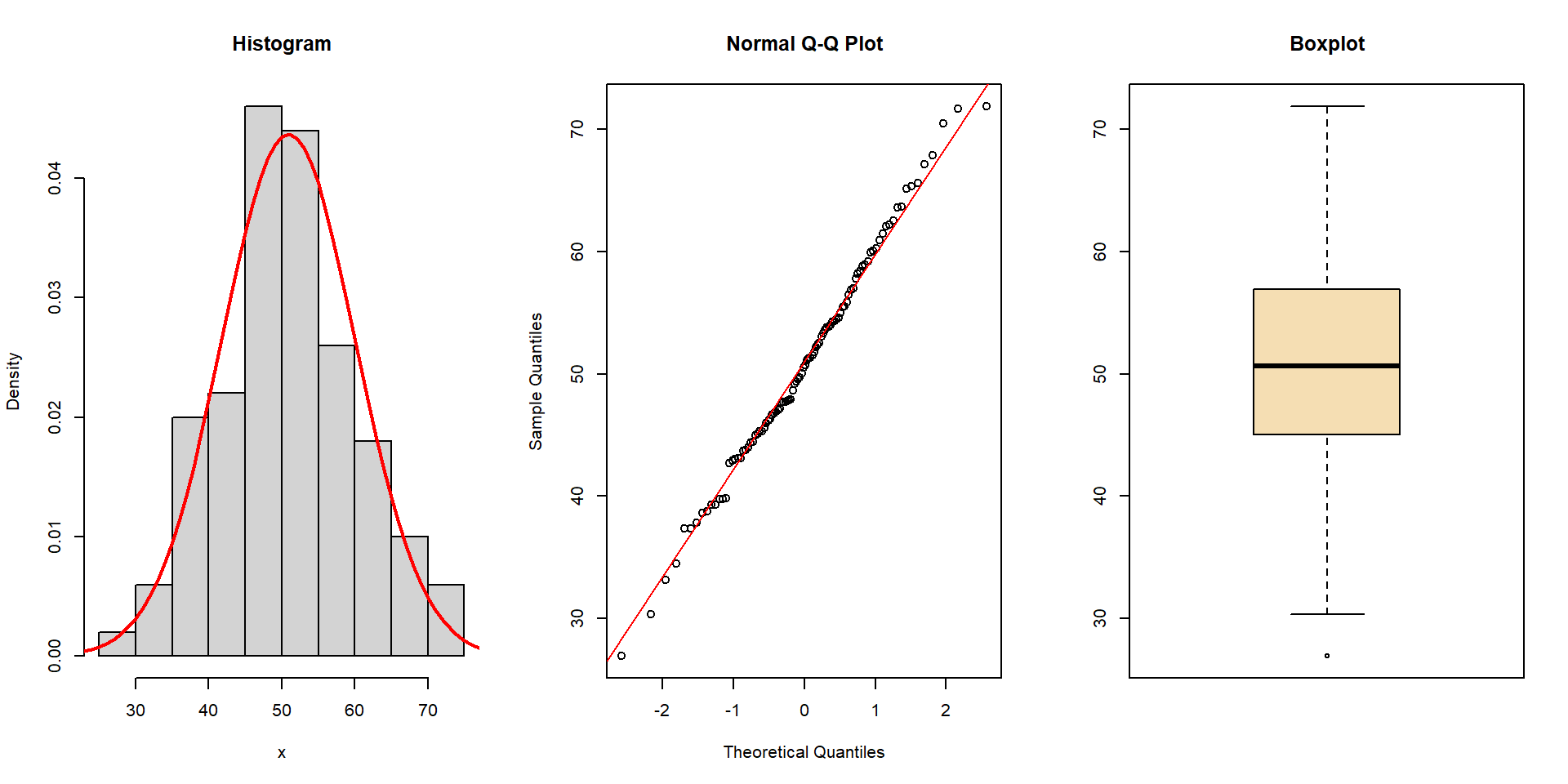
\(x\): theoretical quantiles where a value should be found if the distribution is normal
\(y\): normalized and ordered measured values (\(z\)-scores)
scaled in the unit of standard deviations
normal distribution if the points follow a straight line
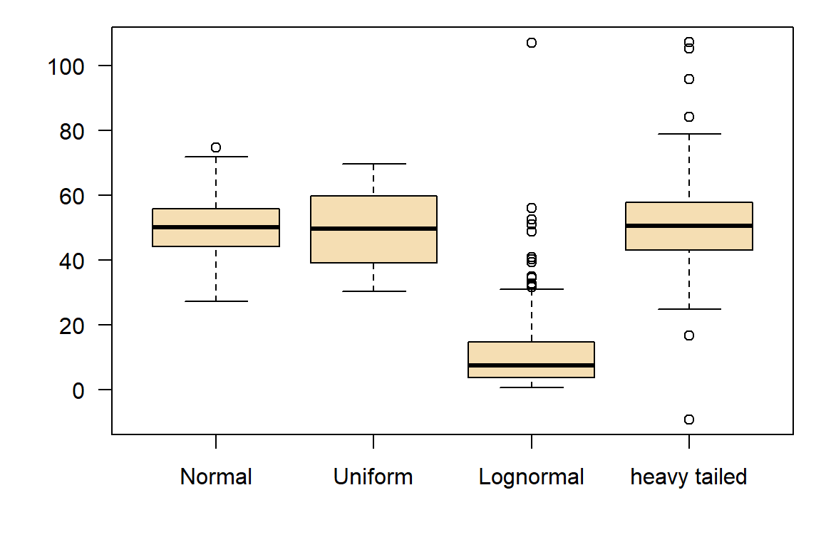
Checking distributions for descriptive purposes
In some disciplines, such as hydrology, it is occasionally necessary to know which distribution type best describes a dataset. This is especially critical for Extreme Value Analysis (e.g., the 100-year flood), as the Central Limit Theorem (CLT) does not apply here.
distribution free (does not require normal distribution),
detects any dependence,
not much affected by outliers.
Disadvantages:
certain information loss due to ranking,
no information about type of dependency,
no direct relationship to coefficient of determination.
Conclusion: \(r_s\) is nevertheless highly recommended!
Correlation coefficients in R
Pearson’s product-moment correlation coefficient
Spearman’s rank correlation coefficient
x <-c(1, 2, 3, 5, 7, 9)y <-c(3, 2, 5, 6, 8, 11)cor.test(x, y, method="pearson")
    Pearson's product-moment correlation

data:  x and y
t = 7.969, df = 4, p-value = 0.001344
alternative hypothesis: true correlation is not equal to 0
95 percent confidence interval:
 0.7439930 0.9968284
sample estimates:
      cor
0.9699203
If linearity or normality of residuals is doubtful, use a rank correlation
cor.test(x, y, method="spearman")
    Spearman's rank correlation rho

data:  x and y
S = 2, p-value = 0.01667
alternative hypothesis: true rho is not equal to 0
sample estimates:
      rho
0.9428571
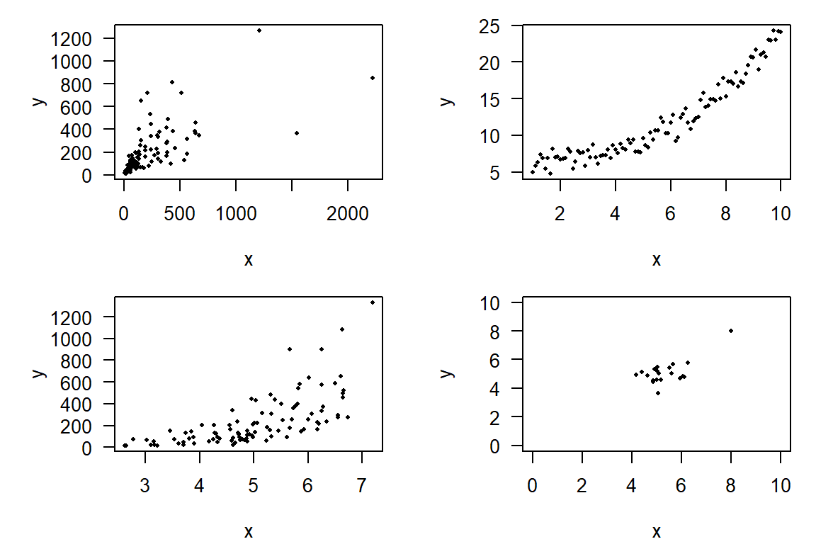
Problematic cases
Outlook: More than two independent variables
Multiple correlation
Example: Chl-a=\(f(x_1, x_2, x_3, \dots)\), where \(x_i\) = biomass of the \(i\)th phytoplankton species.
multiple correlation coefficient
partial correlation coefficient
attractive method \(\leftrightarrow\) but difficult in practice:
“independent” variables may correlate with each other (multi-collinearity) \(\Rightarrow\) bias of the multiple \(r\).
non-linearities are even more difficult to handle than in the two-sample case.
Recommendation:
Use multivariate methods (NMDS, PCA, …) for a first overview,
apply multiple regression with care and use process knowledge.
References
Hubbard, R. (2004). Alphabet soup: Blurring the distinctions between p’s and a’s in psychological research. Theory & Psychology, 14(3), 295–327. https://doi.org/10.1177/0959354304043638
Zimmerman, D. W. (2004). A note on preliminary tests of equality of variances. British Journal of Mathematical and Statistical Psychology, 57(1), 173–181. https://doi.org/10.1348/000711004849222