| number | 1 | 2 | 3 | 4 | 5 | 6 | 7 | 8 | 9 |
| freqency | 0 | 1 | 5 | 5 | 6 | 4 | 12 | 3 | 3 |
04-Distributions
Applied Statistics – A Practical Course
2026-01-28
What is your favorite number?
In a classroom experiment, students of an international course were asked for their favorite number from 1 to 9.
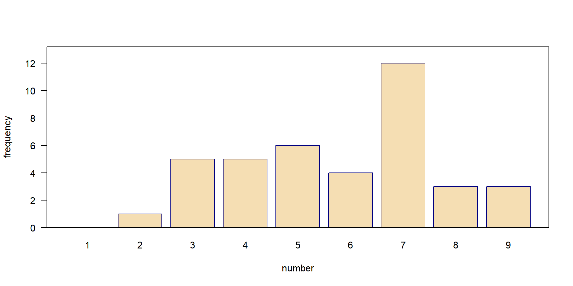
The resulting distribution is:
- empirical: data from an experiment
- discrete: only discrete numbers (1, 2, 3 …, 9) possible, no fractions
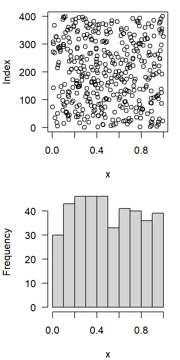
Continuos uniform distribution \(\mathbf{U}(0, 1)\)
- same probability of occurence in a given interval
- e.g. \([0, 1]\)
- in R:
runif, random, uniform
runif(10) [1] 0.8753059 0.4118662 0.4445771 0.7118754 0.1885591 0.7365963 0.9926510
[8] 0.7101854 0.8830810 0.2917783
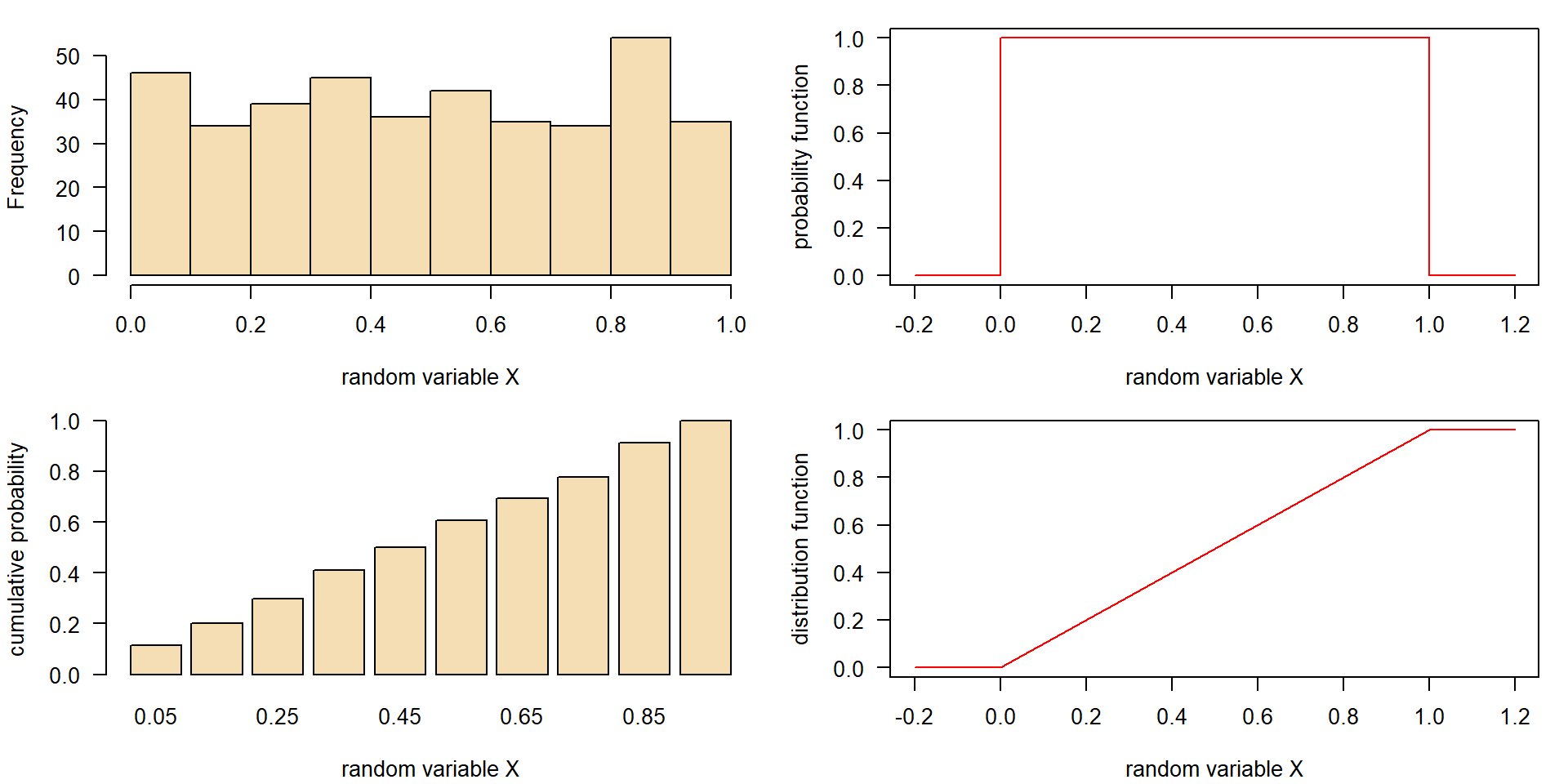
- binning: subdivide values into classes
Density function of \(\mathbf{U}(x_{min}, x_{max})\)
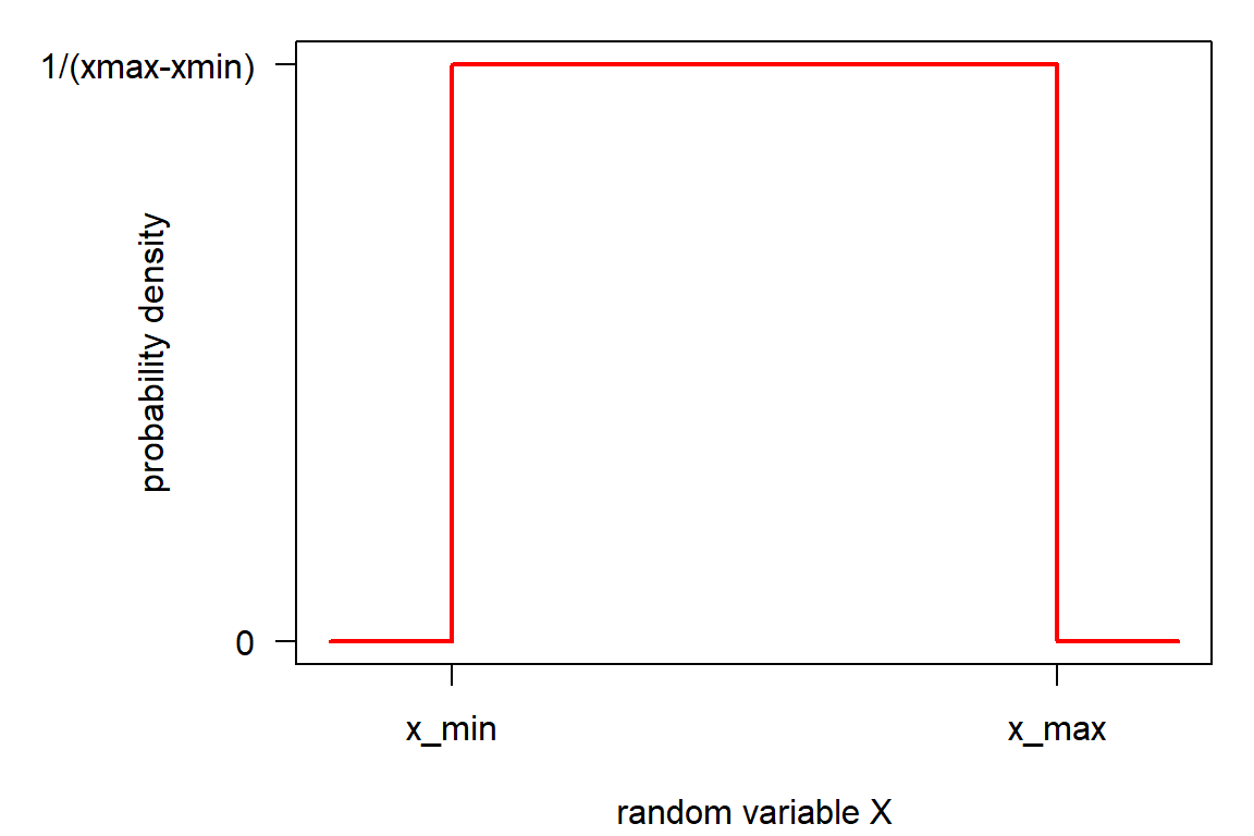
- density \(f(X)\), sometimes abbreviated as “pdf” (probability density function):
\[ f(x) = \begin{cases} \frac{1}{x_{max}-x_{min}} & \text{for } x \in [x_{min},x_{max}] \\ 0 & \text{otherwise} \end{cases} \]
- area under the curve (i.e. the integral) = 1.0
- 100% of the events are between \(-\infty\) and \(+\infty\)
and for \(\mathbf{U}(x_{min}, x_{max})\) in the interval \([x_{min}, y_{max}]\)
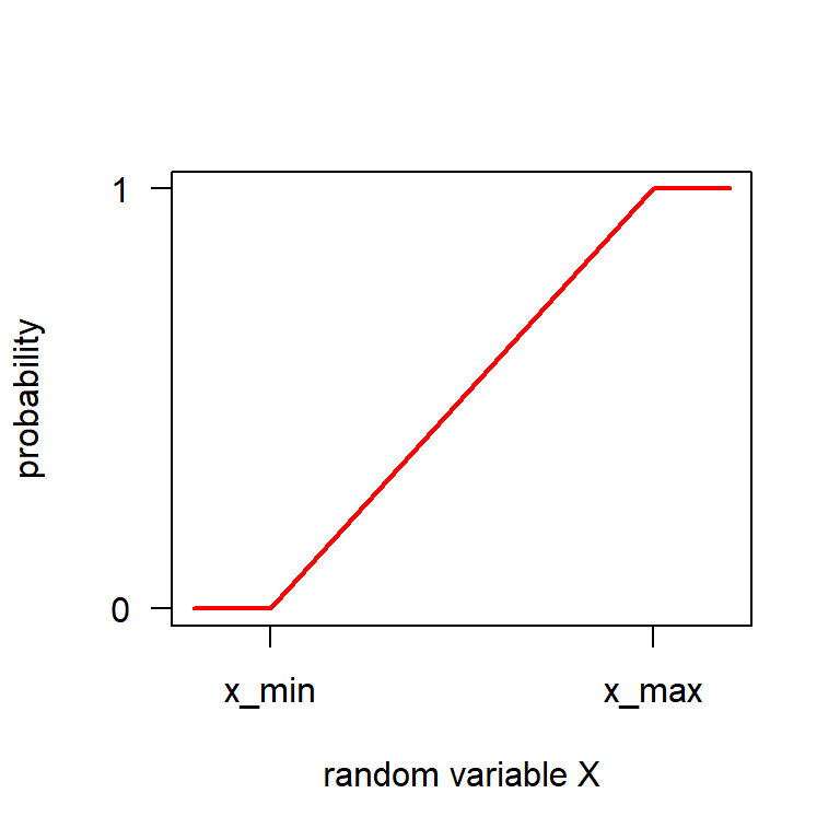
Cumulative distribution function of \(\mathbf{U}(x_{min}, x_{max})\)
The cdf is the integral of the density function:
\[ F(x) =\int_{-\infty}^{x} f(x) dx \] The total area (total probability) is \(1.0\):
\[ F(x) =\int_{-\infty}^{+\infty} f(x) dx = 1 \]
For the uniform distribution, it is:
\[ F(x) = \begin{cases} 0 & \text{for } x < x_{min} \\ \frac{x-x_{min}}{x_{max}-x_{min}} & \text{for } x \in [x_{min},x_{max}] \\ 1 & \text{for } x > x_{max} \end{cases} \]
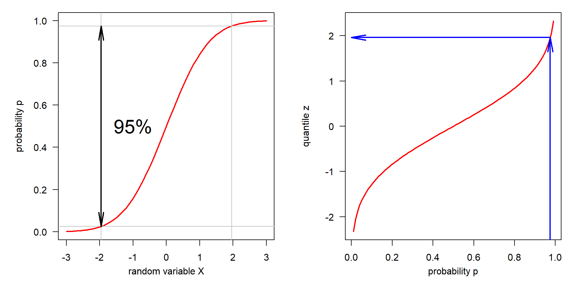
Quantile function
… the inverse of the cumulative distribution function.
Cumulative distribution function
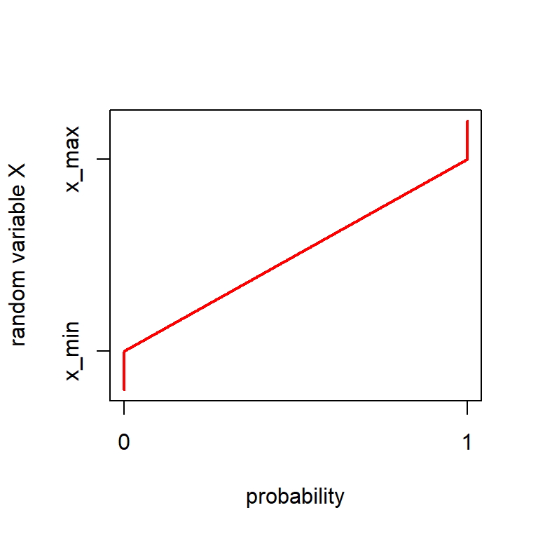
Quantile function
Example: In which range can we find 95% of a uniform distribution \(\mathbf{U}(40,60)\)?
Summary: Uniform distribution
The normal distribution \(\mathbf{N}(\mu, \sigma)\)
- of high theoretical importance due to the central limit theorem (CLT)
- results from adding a large number of random values of same order of magnitude.
The density function of the normal distribution is mathematically beautiful.
\[ f(x) = \frac{1}{\sigma\sqrt{2\pi}} \, \mathrm{e}^{-\frac{(x-\mu)^2}{2 \sigma^2}} \]

C.F. Gauss, Gauss curve and formula on a German DM banknote from 1991–2001 (Wikipedia, CC0)
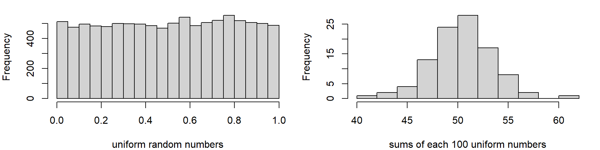
The central limit theorem (CLT)
Sums of a large number \(n\) of independent and identically distributed random values are normally distributed, independently on the type of the original distribution.
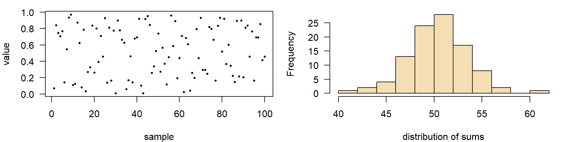
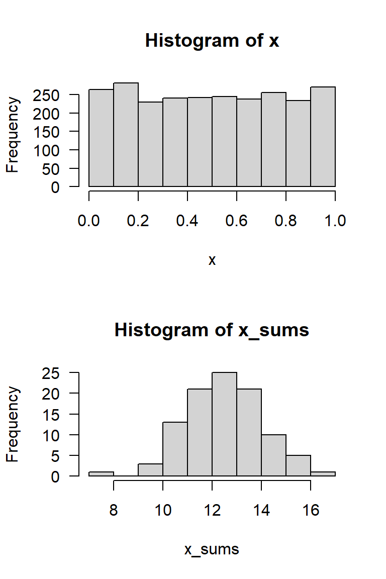
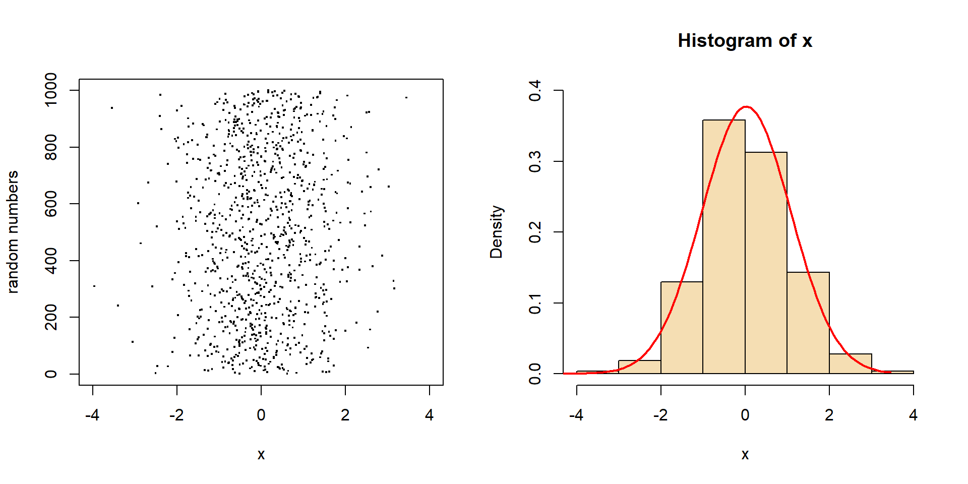
A Simulation experiment
- generate a matrix with 100 rows and 25 columns of uniformly distributed random numbers
- compute the row sums
par(mfrow=c(2, 1), las=1)
set.seed(42)
x  <- matrix(runif(25 * 100), ncol = 25)

# View(x) # uncomment this to show the matrix

x_sums <- rowSums(x)
hist(x)
hist(x_sums)
\(\rightarrow\) row sums are approximately normal distributed
Random numbers and density function
Density and quantiles of the standard normal
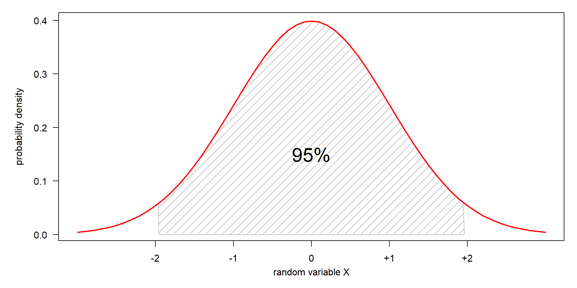
- in theory, 50% of the values are below and 50% above the mean value
- 95% are between \(\pm 2 \sigma\)
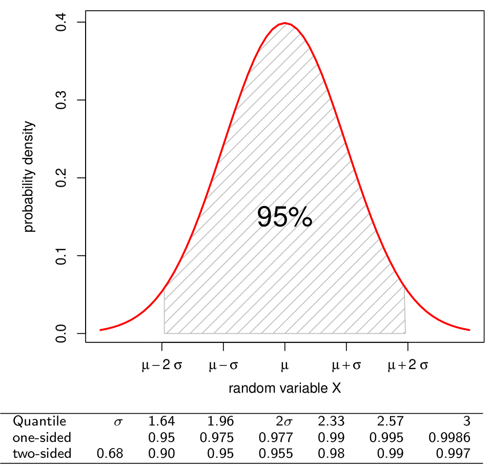
Density and quantiles of the standard normal
Cumulative distribution function – Quantile function
| Quantile | 1 | 1.64 | 1.96 | 2.0 | 2.33 | 2.57 | 3 | \(\mu \pm z\cdot \sigma\) |
|---|---|---|---|---|---|---|---|---|
| one-sided | 0.95 | 0.975 | 0.977 | 0.99 | 0.995 | 0.9986 | \(1-\alpha\) | |
| two-sided | 0.68 | 0.90 | 0.95 | 0.955 | 0.98 | 0.99 | 0.997 | \(1-\alpha/2\) |
Standard normal, scaling and shifting
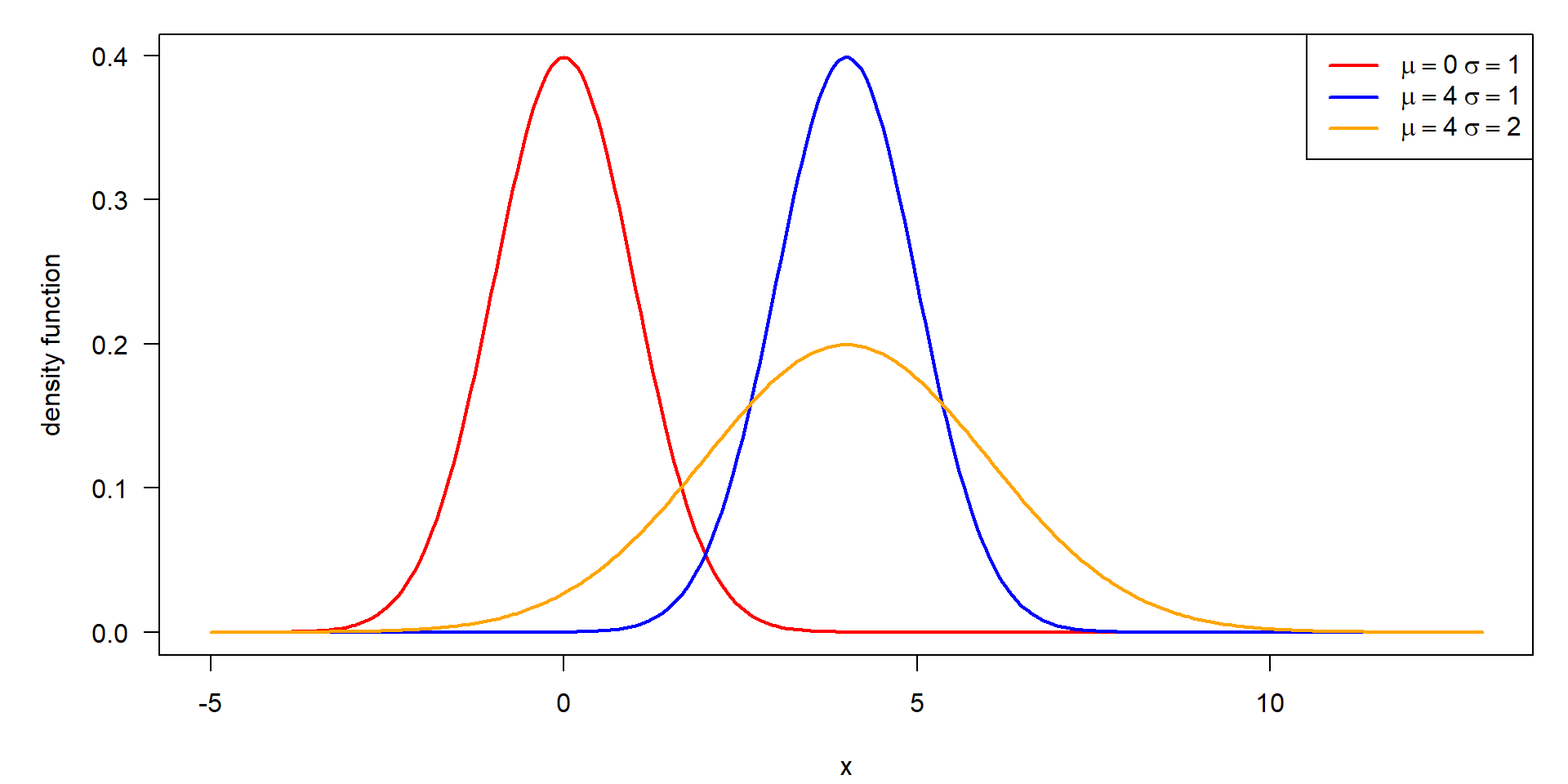
- \(\mu\) is the shift parameter that moves the whole bell shaped curve along the \(x\) axis
- \(\sigma\) is the scale parameter to stretch or compress in the direction of \(x\)
Standardization (\(z\)-transformation)
Any normal distribution can be shifted scaled to form a standard normal with \(\mu=0, \sigma=1\)
Normal distribution
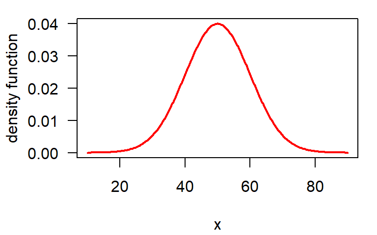
\[ f(x) = \frac{1}{\sigma\sqrt{2\pi}} \, \mathrm{e}^{-\frac{(x-\mu)^2}{2 \sigma^2}} \]
\[
z = \frac{x-\mu}{\sigma}
\] \(\longrightarrow\) \(\longrightarrow\) \(\longrightarrow\)
Standard normal distribution
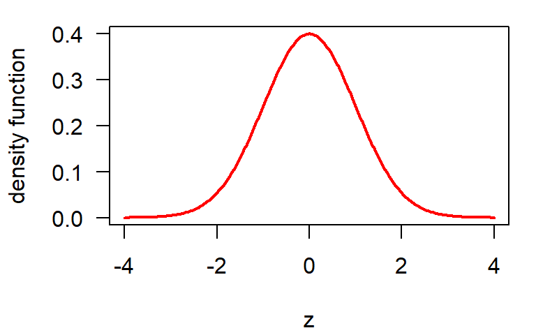
\[ f(x) = \frac{1}{\sqrt{2\pi}} \, \mathrm{e}^{-\frac{1}{2}x^2} \]
t-Distribution \(\mathbf{t}(x, df)\)
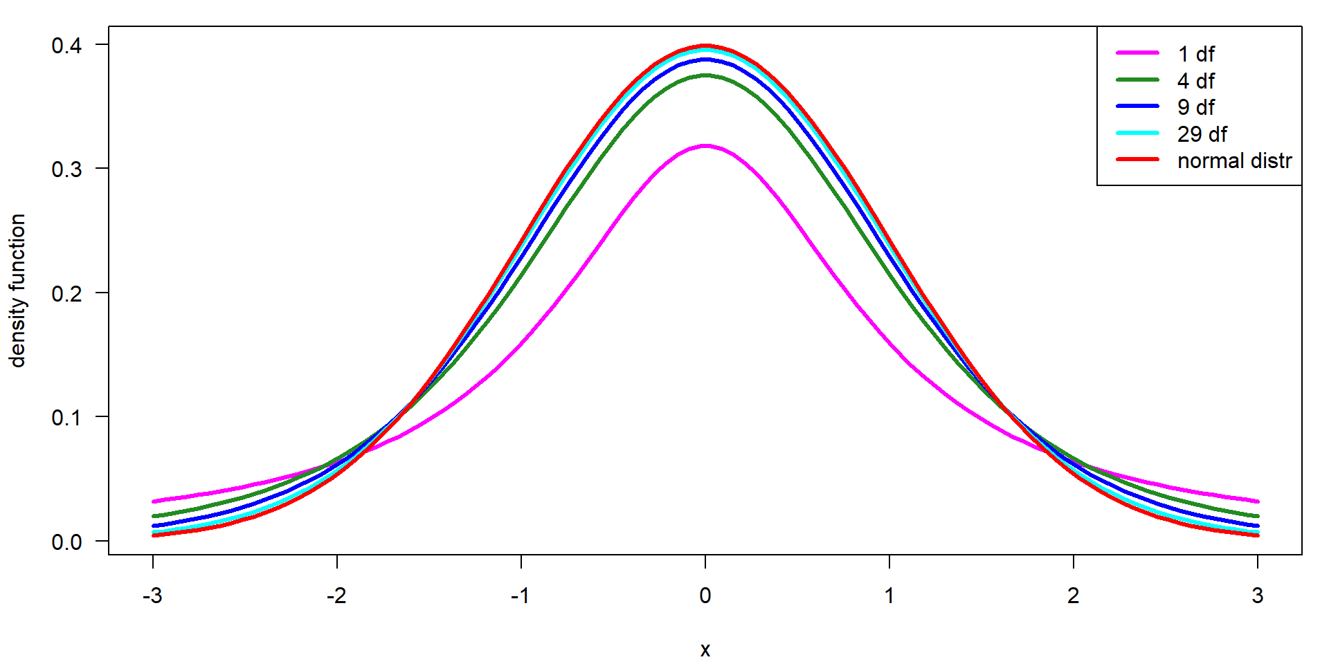
- additional parameter “degrees of freedom” (df)
- used for confidence intervals and statistical tests
- converges to the normal distribution for \(df \rightarrow \infty\)
Dependency of the t-value on the number of df
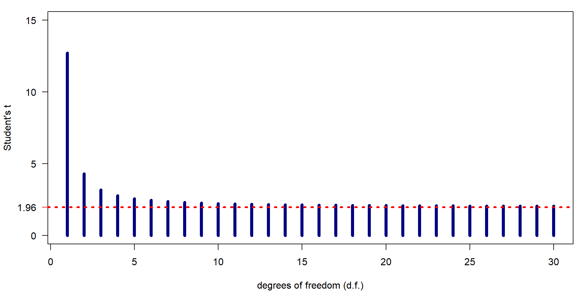
| df | 1.00 | 4.00 | 9.00 | 19.00 | 29.00 | 99.00 | 999.00 |
| t | 12.71 | 2.78 | 2.26 | 2.09 | 2.05 | 1.98 | 1.96 |
Logarithmic normal distribution (lognormal)
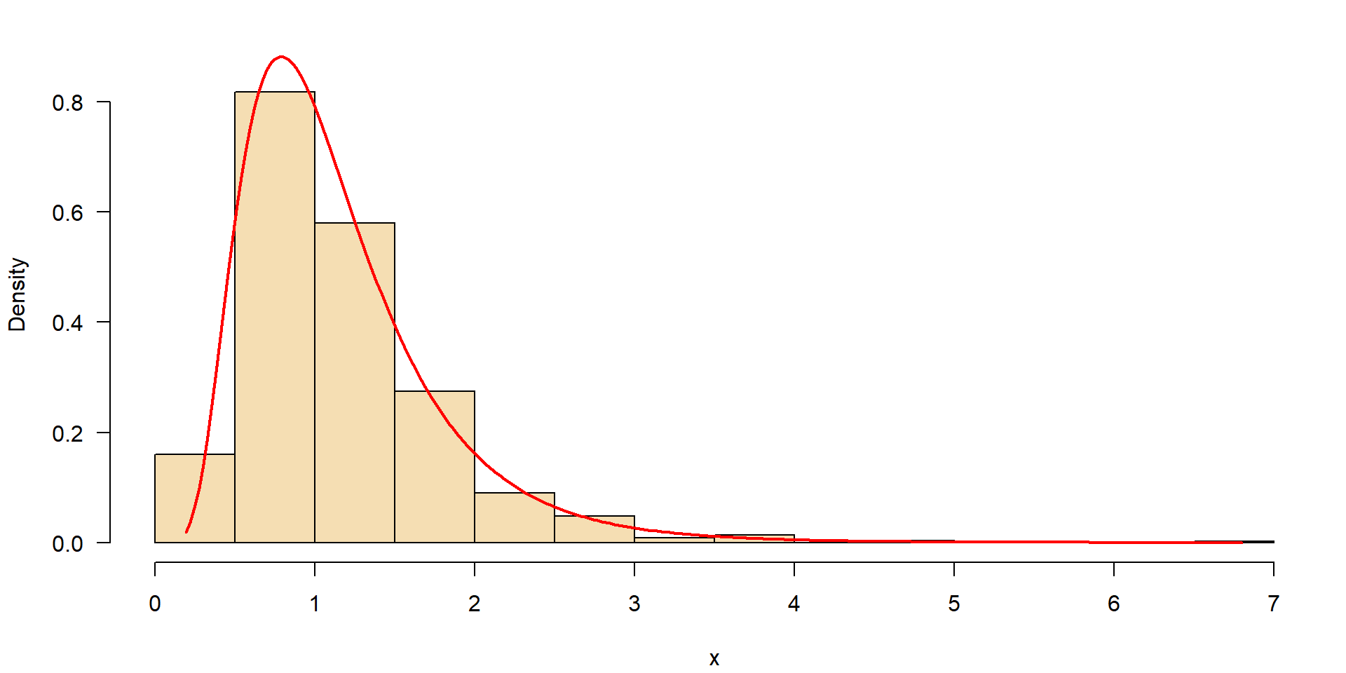
- many processes in nature do not follow a normal distribution
- limited by zero on the left side
- large extreme values on the right side
Examples: discharge of rivers, nutrient concentrations, algae biomass in a lakes
Parent distribution of the lognormal
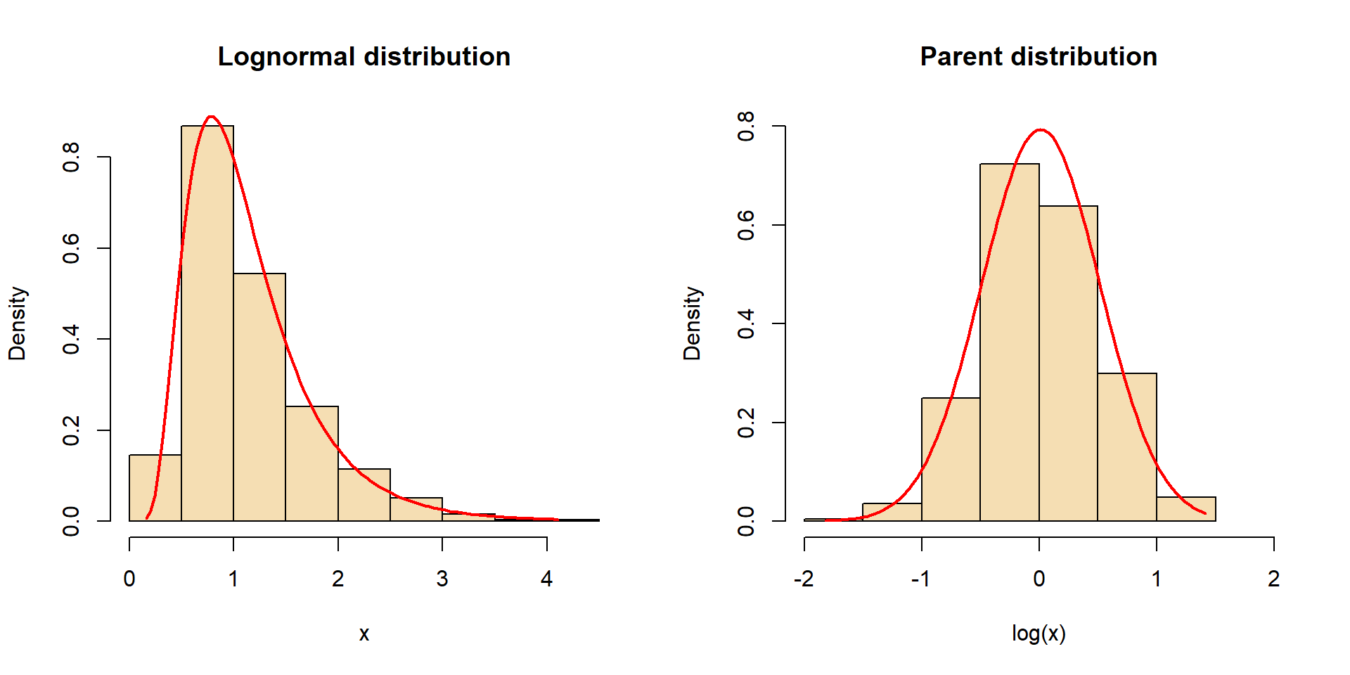
- log from values of a lognormal distribution \(\rightarrow\) normal parent distribution.
- lognormal distribution is described by parameters of log-transformed data \(\bar{x}_L\) and \(s_L\)
- the the antilog of \(\bar{x}_L\) is the geometric mean
Binomial distribution
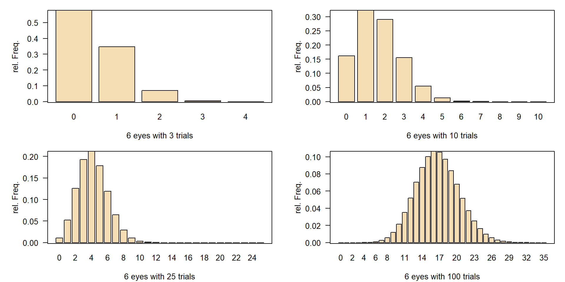
- number of successful trials out of \(n\) total trials with success probability \(p\).
- How many “6” with probability \(1/6\) in 3 trials?
- medicine, toxicology, comparison of percent numbers
- similar, but without replacement: hypergeometric distribution in lottery
Poisson distribution
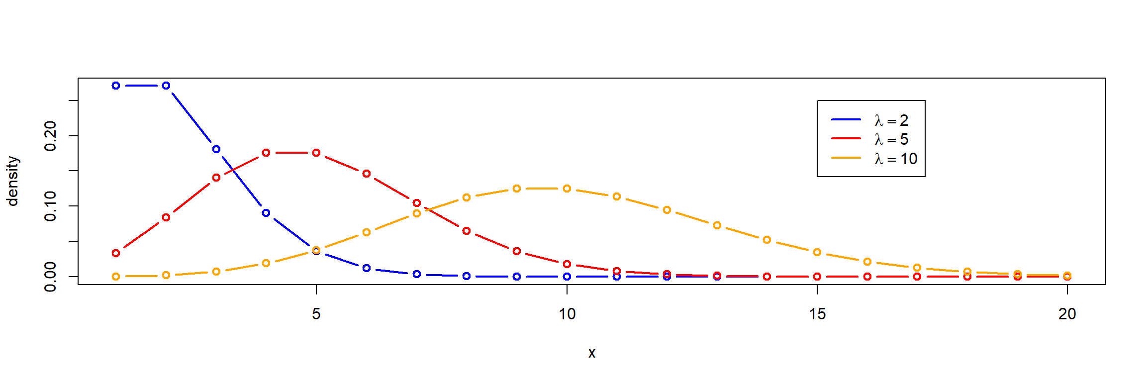
- distribution of rare events, a discrete distribution
- mean and variance are equal (\(\mu = \sigma^2\)), resulting parameter “lambda” (\(\lambda\))
- Examples: bacteria counting on a grid, waiting queues, failure models
Quasi-poisson if \(\mu \neq \sigma^2\)
- If \(s^2 > \bar{x}\): overdispersion
- if \(s^2 < \bar{x}\): underdispersion
Confidence interval
– depends only on \(\lambda\) resp. the number of counted units (\(k\))
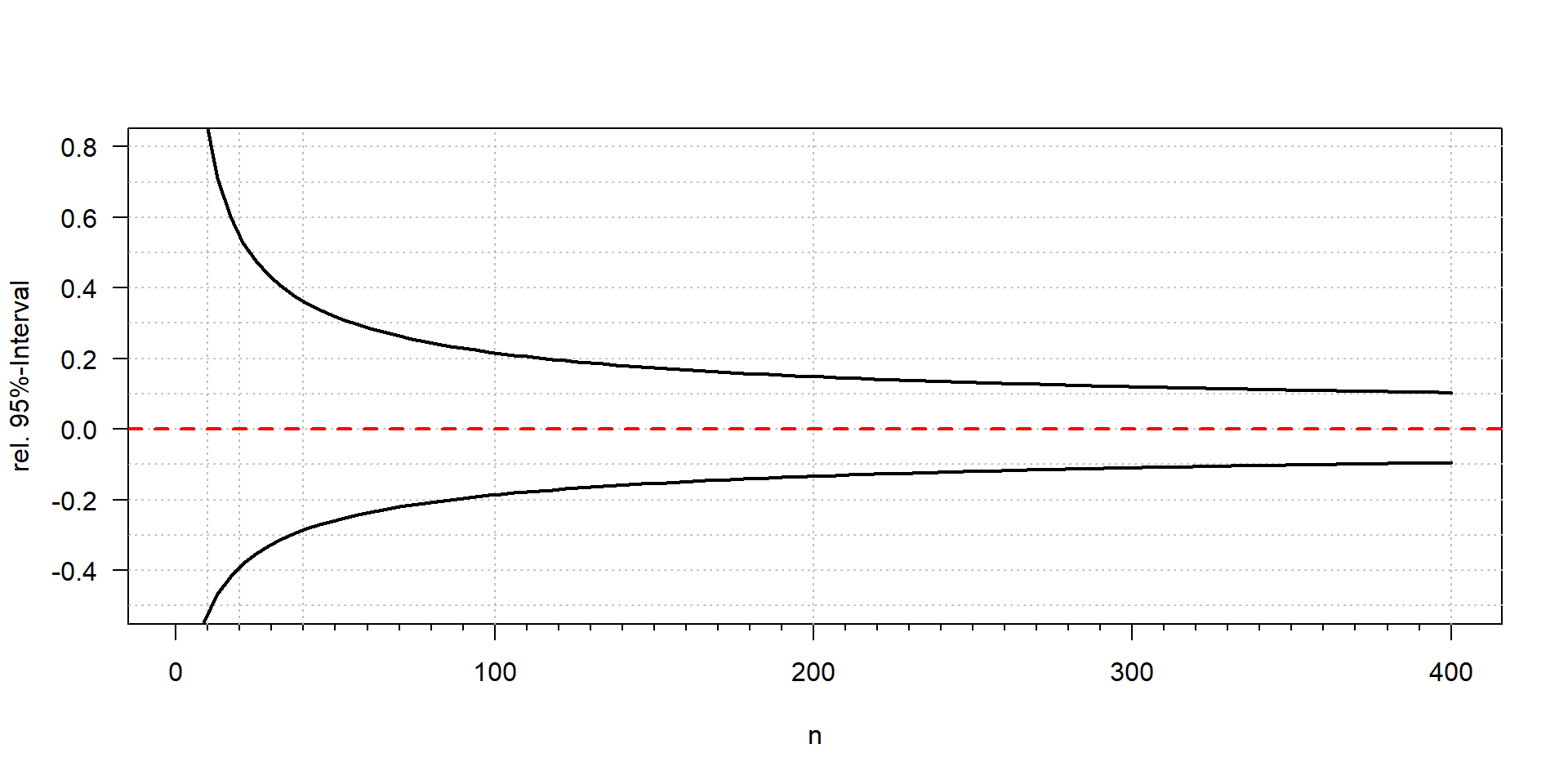
Typical error of cell counting: 95% confidence interval
| counts | 2 | 3 | 5 | 10 | 50 | 100 | 200 | 400 | 1000 |
| lower | 0 | 1 | 2 | 5 | 37 | 81 | 173 | 362 | 939 |
| upper | 7 | 9 | 12 | 18 | 66 | 122 | 230 | 441 | 1064 |
Remember: The central limit theorem (CLT)
Sums of a large number \(n\) of independent and identically distributed random values are normally distributed, independently on the type of the original distribution.
- we can use methods assuming normal normal distribution for non-normal data
- if we have a large data set
- if the original distribution is not “too skewed”
- required number \(n\) depends on the skewness of the original distribution
Reason: Methods like t-test or ANOVA are based on mean values.
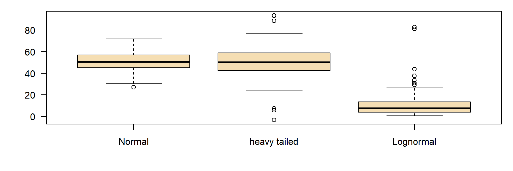
Extreme values in boxplots
extreme values outside the whiskers if more than 1.5 times distant from the box limits, compared to the width of the interquartile box.
sometimes called “outliers”.
I prefer the term “extreme value”, because they can be regular observations from a skewed or heavy tailed distribution.
Example
par(mfrow=c(1, 3), las=1)
elbe <- read.csv("https://tpetzoldt.github.io/datasets/data/elbe.csv")
discharge <- elbe$discharge
boxplot(discharge, main="Boxplot of discharge")
hist(discharge)
hist(log(discharge - 70))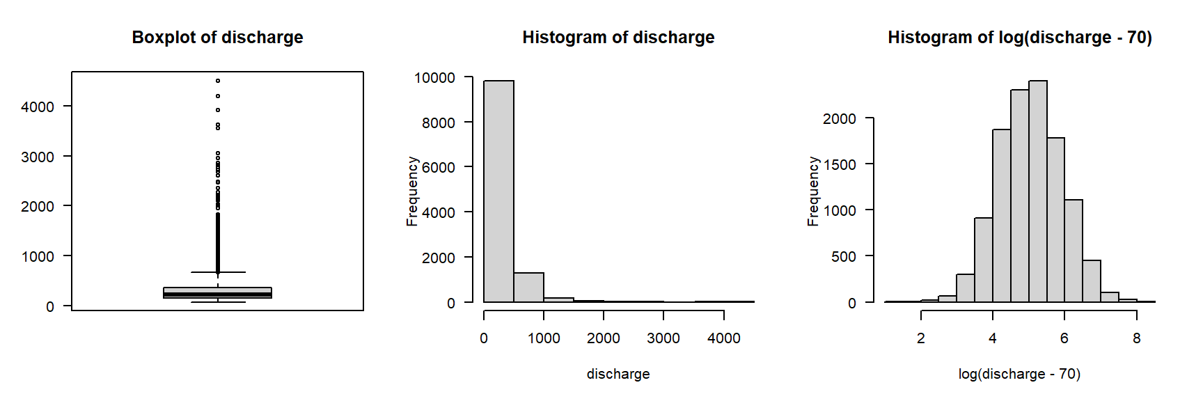
Discharge data of the Elbe River in Dresden in \(\mathrm m^3 s^{-1}\), data source: Bundesanstalt für Gewässerkunde (BFG), see terms and conditions.
- left: large number of extreme values, are these outliers?
- middle: distribution is right-skewed
- right: transformation (3-parametric lognormal) \(\rightarrow\) symmetric distribution, no outliers!