03-Statistical Parameters
Applied Statistics – A Practical Course
2026-01-28
Statistical Parameters
\(\rightarrow\) Remember: calculation of statistical parameters is called estimation
Properties of statistical parameters
- Unbiasedness: the estimation converges towards the true value with increasing \(n\)
- Efficiency a relatively small \(n\) is sufficient for a good estimation
- Robustness the estimation is not much influenced by outliers or certain violations of statistical assumptions
Depending on a particular question, different classes of parameters exist, especially measures of location (e.g. mean, median), variation (e.g. variance, standard deviation) or dependence (e.g. correlation).
Measures of location I
Arithmetic mean
\[
\bar{x} = \frac{1}{n} \cdot {\sum_{i=1}^n x_i}
\]
Geometric mean
\[
G = \sqrt[n]{\prod_{i=1}^n x_i}
\]
more practical: logarithmic form:
\[
G =\exp\Bigg(\frac{1}{n} \cdot {\sum_{i=1}^n \ln{x_i}}\Bigg)
\]
avoids huge numbers that make problems for the computer.
Measures of location II
Harmonic mean
\[
\frac{1}{H}=\frac{1}{n}\cdot \sum_{i=1}^n \frac{1}{x_i} \quad; x_i>0
\]
Example:
You drive with 50km/h to the university and with 100km/h back home.
What is the mean velocity?
Result:
1/((1/50 + 1/100)/2) = 1/((0.02 + 0.01)/2) = 1/0.015 = 66.67
Trimmed mean
- also called “truncated mean”
- compromize between the arithmetic mean and median
- A certain percentage of smallest and biggest values is ignored (e.g. 10% or 25%) before calculating the arithmetic mean
- used also in sports
Example: sample with 20 values, exclude 10% at both sides
0.4, 0.5, 1, 2.5, 2.9, 3.3, 4.1, 4.5, 4.6, 5.3, 5.5, 5.7, 6.8, 7.9, 8.8, 8.9, 9, 9.4, 9.6, 46
\(\rightarrow\) arithmetic mean: \(\bar{x}=7.335\)
\(\rightarrow\) trimmed mean: \(\bar{x}_{t, 0.1}=5.6375\)
- median and trimmed mean are less influenced by outliers and skewnes \(\rightarrow\) more robust
- but somewhat less efficient
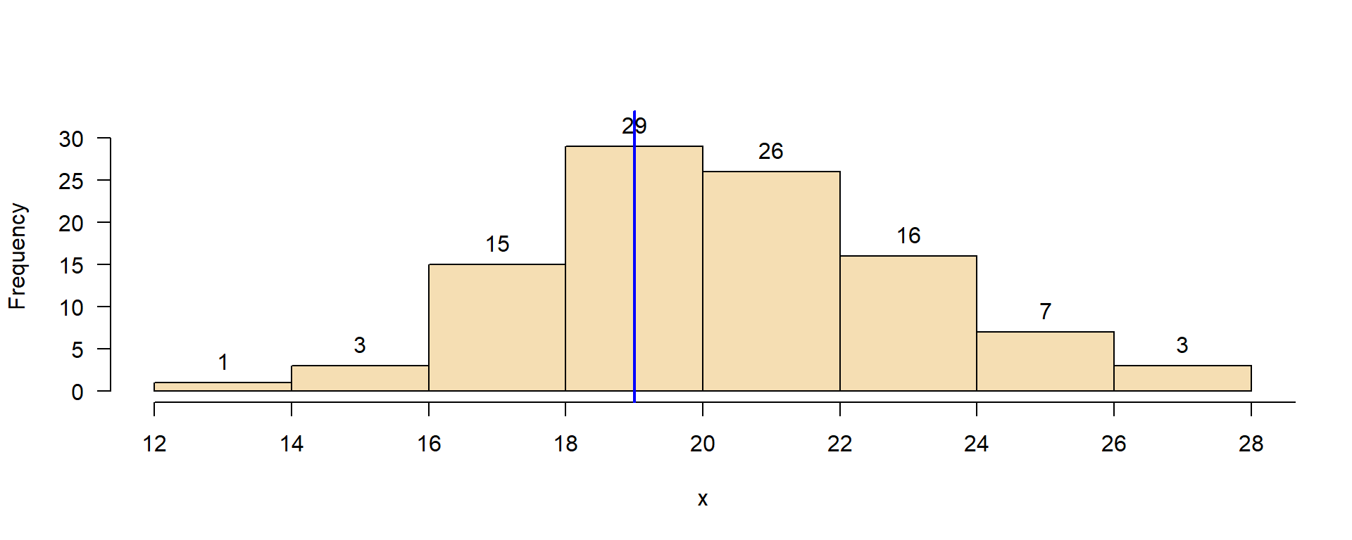
Mode (modal value)
![]()
- most frequent value of a sample
- strict definition only valid for discrete (binary, nominal, ordinal) scales
- extension to continuous scale: binning or density estimation
First guess: middle of most-frequent class.
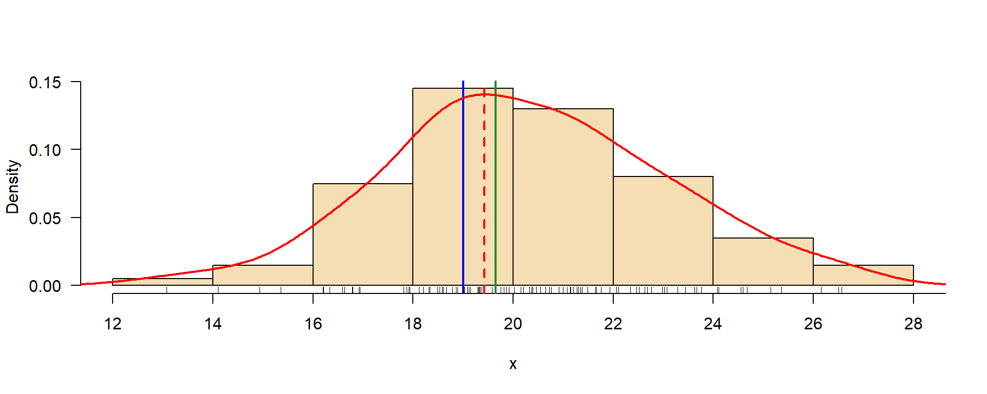
Mode: density estimation
![]()
Somewhat more computer intensive, where the mode is the maximum of a kernel density estimate.
The mode from the density estimate is then \(D=19.42\).
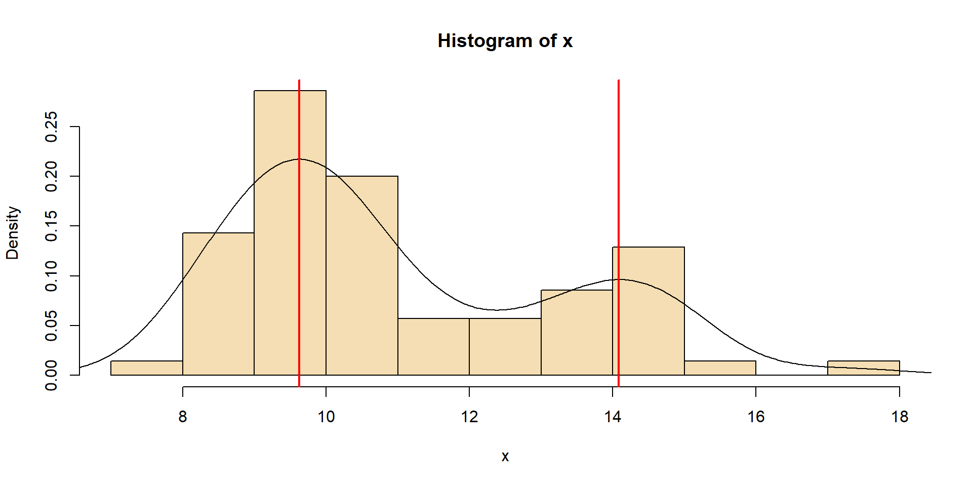
Multi-modal distribution
![]()
Example: fish population with several age classes, cohorts)
Measures of variation
Variance
\[
s^2_x = \frac{SQ}{df}=\frac{\sum_{i=1}^n (x_i-\bar{x})^2}{n-1}
\]
- \(SQ\): sum of squared differences from the mean \(\bar{x}\)
- \(df = n-1\): degrees of freedom, \(n\): sample size
Standard deviation
\[s=\sqrt{s^2}\] \(\rightarrow\) same unit as the mean \(\bar{x}\), so they can be directly compared.
In practice, \(s^2\) is often computed with:
\[
s^2_x = \frac{\sum{(x_i)^2}-(\sum{x_i})^2/n}{n-1}
\]
Coefficient of variation (\(cv\))
Is the relative standard deviation:
\[
cv=\frac{s}{\bar{x}}
\]
- useful to compare variations of different variables, independent of their measurement unit
- only applicable for data with ratio scale, i.e. with an absolute zero (like meters)
- not for variables like Celsius temperature or pH.
Example
Let’s assume we have the discharge of two rivers, one with a \(cv=0.3\), another one with \(cv=0.8\). We see that the 2nd has more extreme variation.
Range
The range measures the difference between maximum and minimum of a sample:
\[
r_x = x_{max}-x_{min}
\]
Disadvantage: very sensitive against outliers.
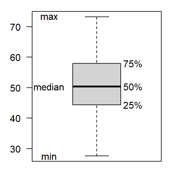
Interquartile range
- IQR or \(I_{50}\) omits smallest and biggest 25%
- sample size of at least 12 values recommended
\[
I_{50}=Q_3-Q_1=P_{75}-P_{25}
\]
Ordered sample
- \(Q_1\), \(Q_3\): 1st and 3rd quartiles
- \(P_{25}, P_{75}\): 25th and 75th percentile
- typically used in boxplots
For normally distributed samples, fixed relationship between \(I_{50}\) and \(s\):
\[
\sigma = E(I_{50}/(2\Phi^{-1}(3/4))) \approx E(I_{50}/1.394) % 2*qnorm(3/4))
\]
where \(\Phi^{-1}\) is the quantile function of the normal distribution.
Standard error of the mean
\[
s_{\bar{x}}=\frac{s}{\sqrt{n}}
\]
- measures the accuracy of the mean
- plays a central role for calculation of confidence intervals and statistical tests
Rule of thumb for a sample size of about \(n > 30\):
- “Two sigma rule”: the true mean is with 95% in the range of \(\bar{x} \pm 2 s_\bar{x}\)
Important
- standard deviation \(s\) measures variability of the sample
- standard error \(s_\bar{x}\) measures accuracy of the mean
More about this will be explained in the next sections.