01-Introduction
Applied Statistics – A Practical Course
2026-01-28
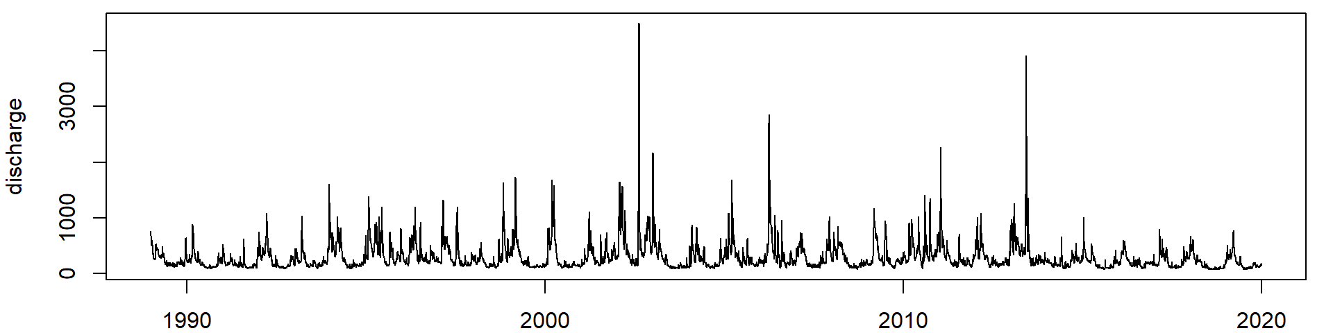
Plot the last 20 years
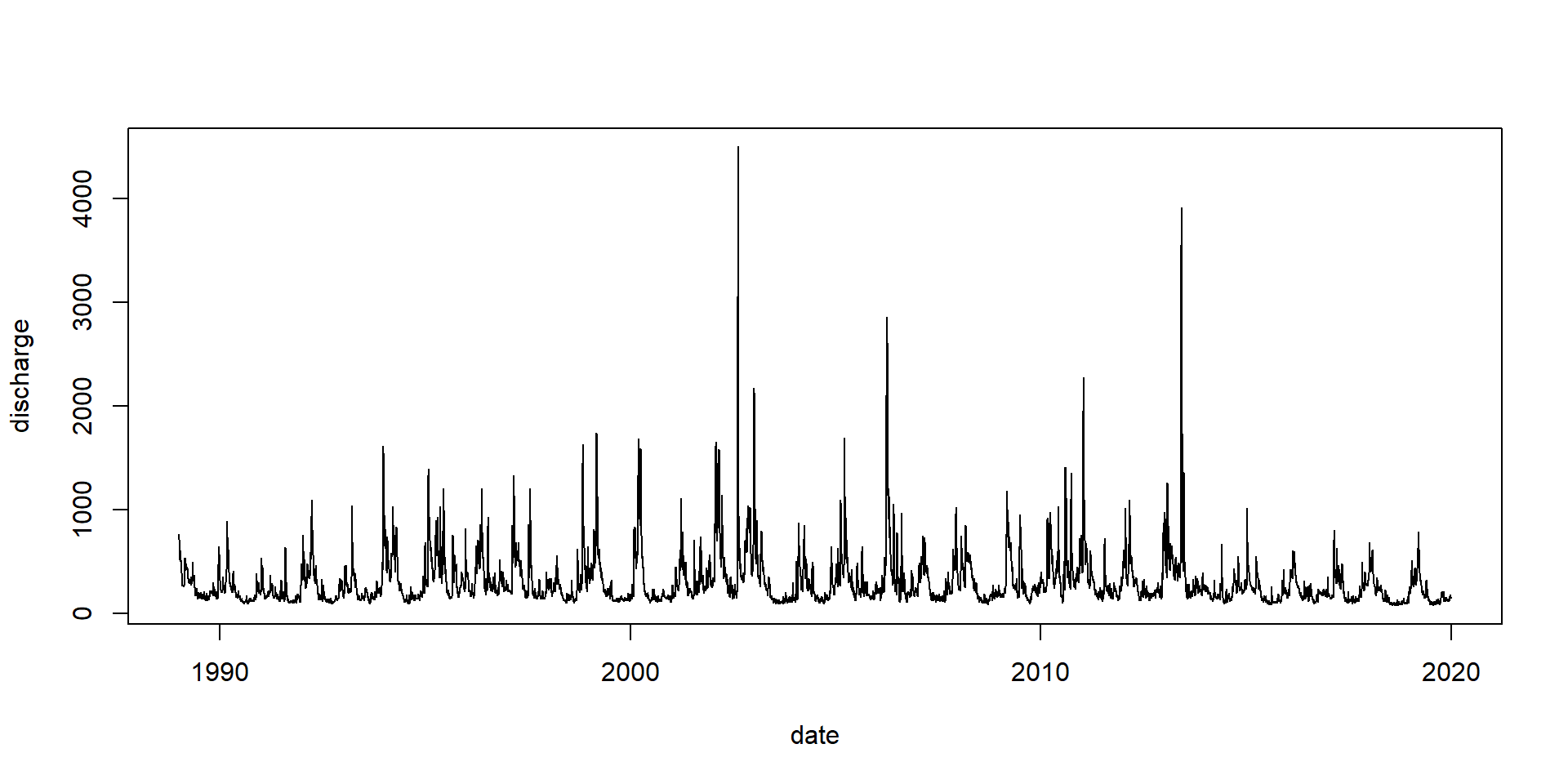
Discharge of the Elbe River, gauge station Dresden, data source BfG
What do these data tell us?

- What is the average discharge? → mean values
- How much variation is in the data? → variance
- How likely are droughts or floods? → distribution
- How precise are our forecasts? → confidence intervals
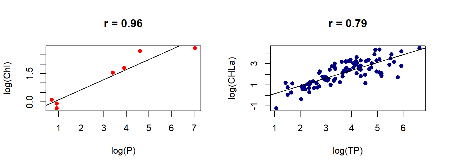
- Which factors influence discharge? → correlations
How to start
- Mean value: 224
- Median value: 224
- Standard deviation: 253
- Range: 2, 4500
Which of these parameters are most appropriate?
Graphics
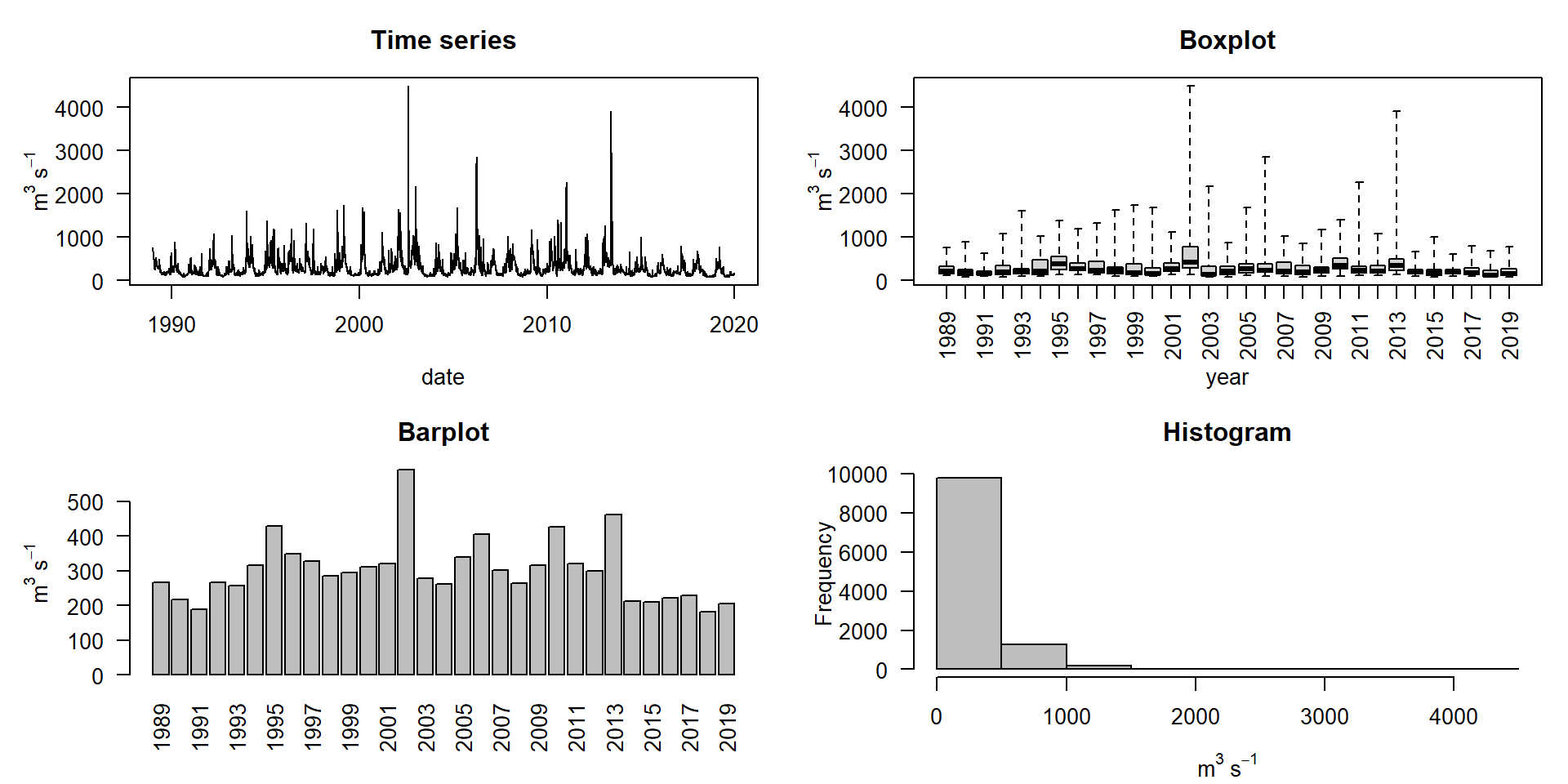
Boxplots
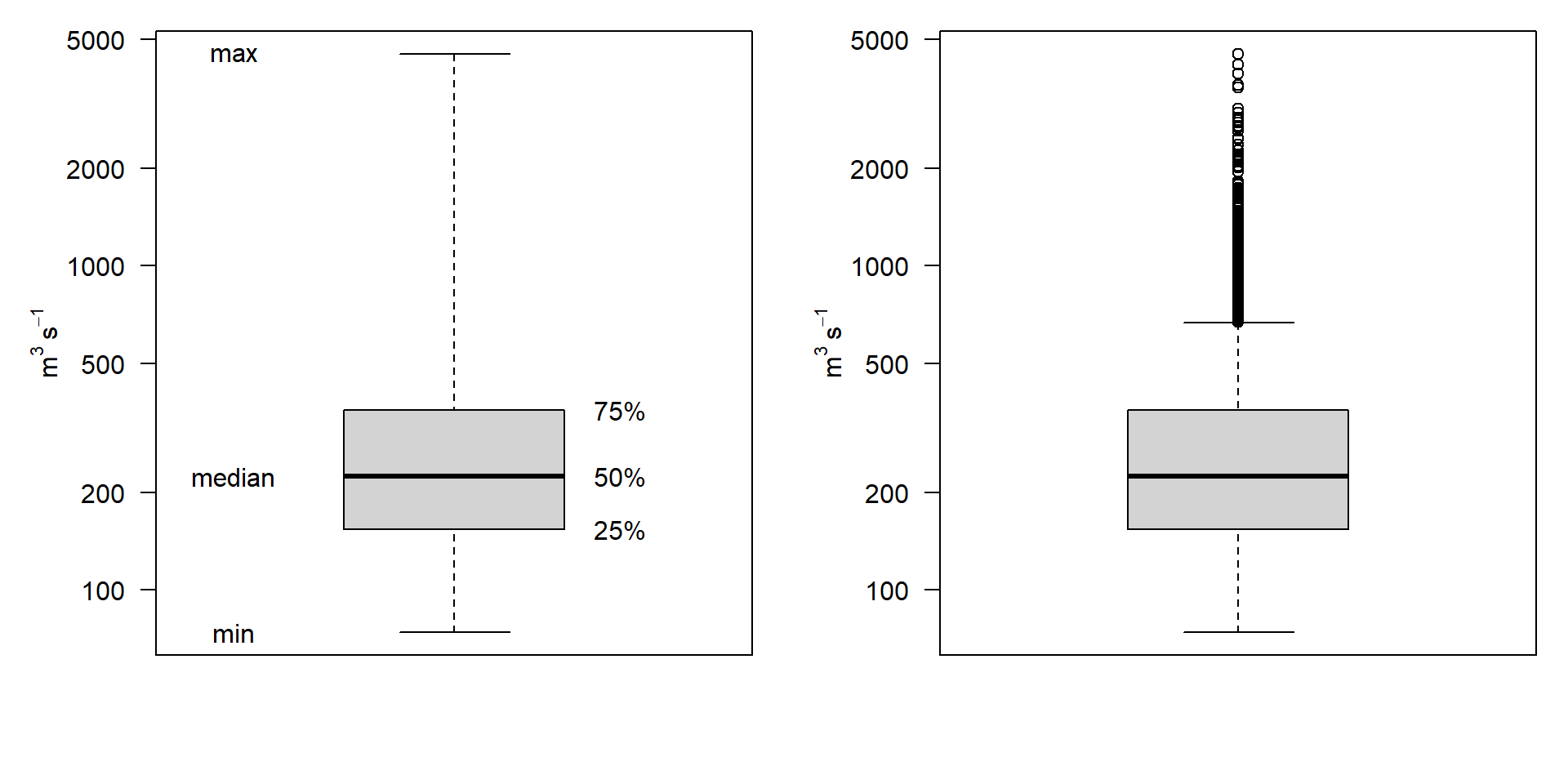
- Note the log scale of y!
- In the right version, whiskers extend to the most extreme data point which is no more than 1.5 times the interquartile range from the box.
Example: Compare two mean values
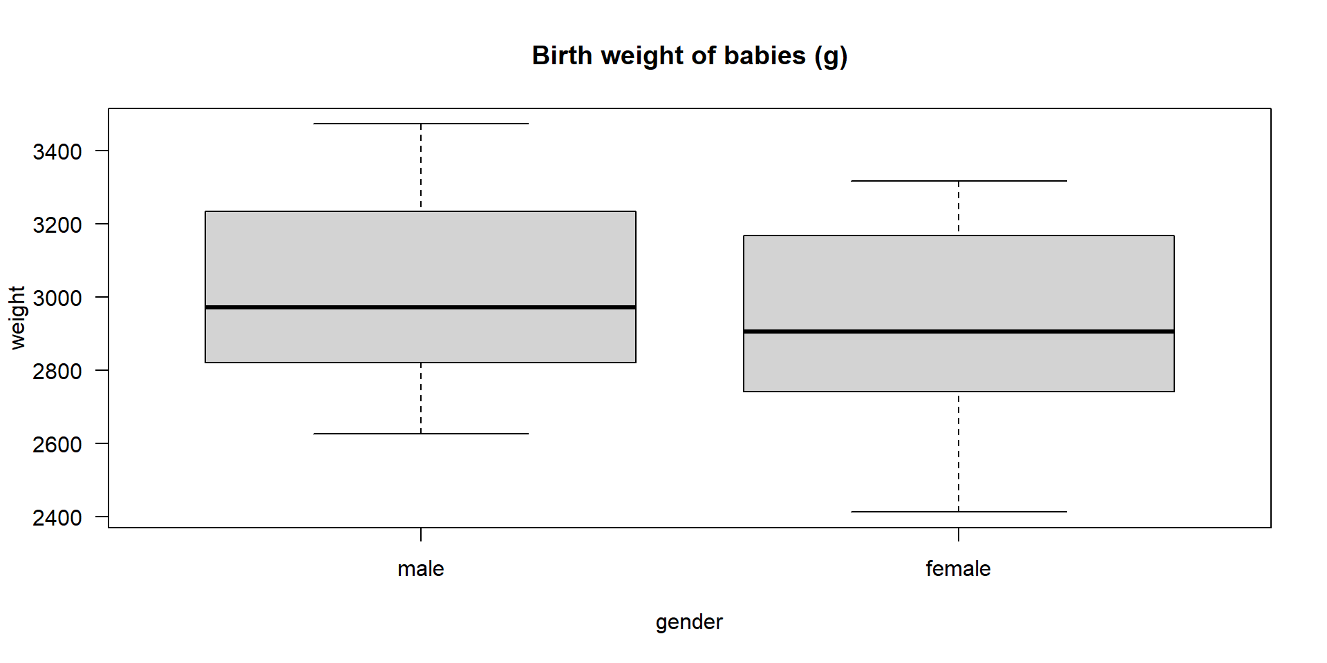
- A given data set (Dobson, 1983) contains the birth weight (in g) of 12 boys and 12 girls.
- Has the weight difference something to do with the gender of the babies or is it a purely random fluctuation?
Computing
Required software
- A spreadsheet program, Excel or LibreOffice https://www.libreoffice.org/
- The R system for data analysis and graphics https://www.r-project.org
- RStudio for making R more user-friendly https://posit.co/download/rstudio-desktop/
Why R?
- Statisticians call it “lingua franca” in computational statistics.
- Extremely powerful
- No other system has so much statistics
- Used in statistical research
- Free (OpenSource)
- Free to use
- Free to modify
- Free to contribute
- Less complicated than its first appearance:
- Yes, it needs command line programming
- but: already a single line can do much
- huge number of books and online scripts
In contrast to other systems Copy & Paste is allowed! – just cite it.