S <-c(25, 25, 10, 10, 5, 5, 2.5, 2.5, 1.25, 1.25)
V <-c(0.0998, 0.0948, 0.076, 0.0724, 0.0557,
      0.0575, 0.0399, 0.0381, 0.017, 0.0253)
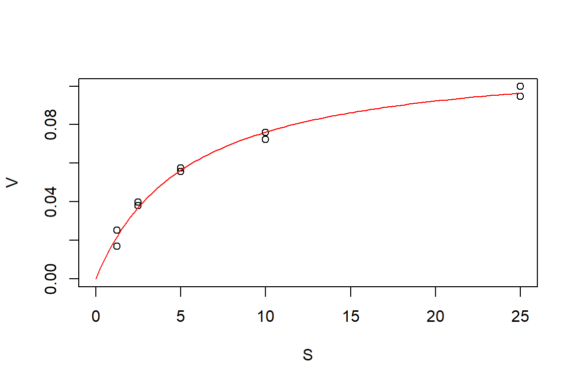
model_fit<-nls(V ~ SSmicmen(S, Vm, K))

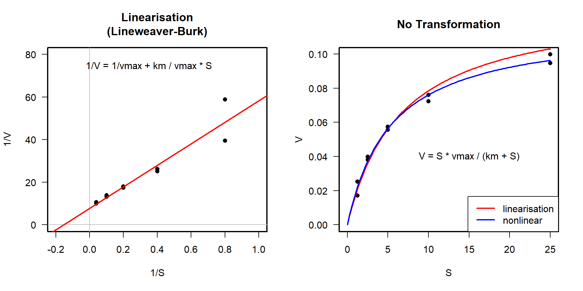
par(mfrow=c(1,2), las=1, lwd=2)
## Lineweaver-Burk
x <- 1/S; y <- 1/V

plot(x, y, xlab="1/S", ylab="1/V", xlim=c(-0.2,1), ylim=c(0, 80), pch=16,
  main="Linearisation\n(Lineweaver-Burk)")
abline(h=0, lwd=1, col="grey")
abline(v=0, lwd=1, col="grey")
m <- lm(y ~ x)
abline(m, col = "red")
Vm_l <- 1/coef(m)[1]
Km_l <- coef(m)[2] * Vm_l
#legend("topleft", c("vmax = 1/intercept", "km = slope * vmax"),
#        box.lwd=1, bg="white")
text(0.35, 75, "1/V = 1/vmax + km / vmax * S")

## retransformed, both together
plot(S, V, xlim = c(0, max(S)),ylim=c(0, max(V)), pch=16, main="No Transformation")
x1 <-seq(0, 25, length=100)
lines(x1, Vm_l * x1 / (Km_l + x1), col="red")
lines(x1, predict(model_fit, data.frame(S=x1)), col="blue")
legend("bottomright", legend=c("linearisation", "nonlinear"),
       box.lwd=1, lwd=2, col=c("red", "blue"))
text(15, 0.04, "V = S * vmax / (km + S)")
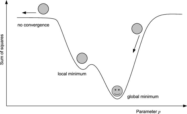
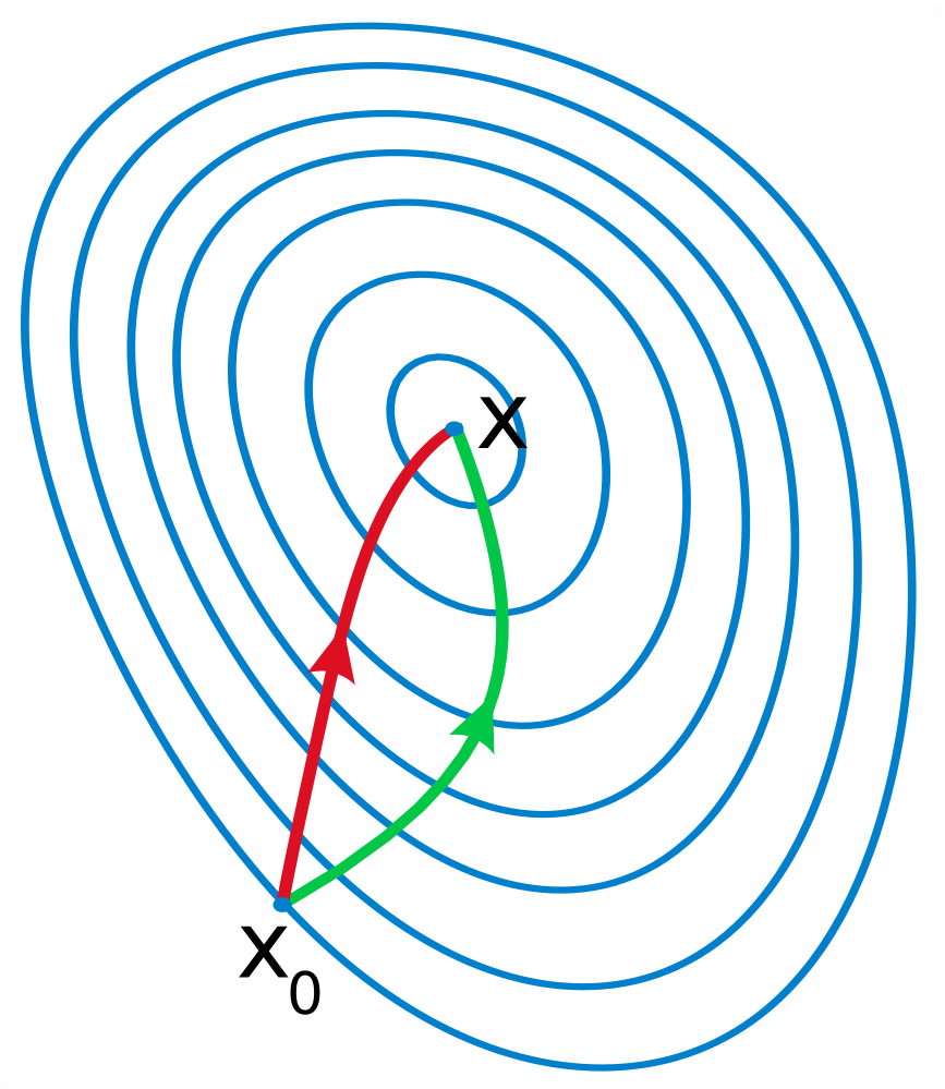 Die Newton-Methode (